Statistical Thinking: Confidence Intervals, Bayes' Theorem, and Replication

Experiment Repeated 100 Times

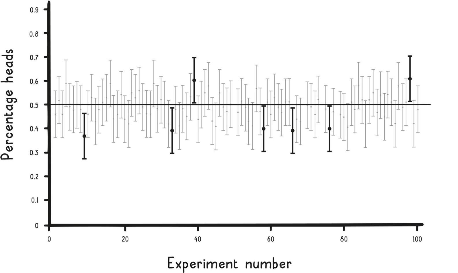
Error bars are not always confidence intervals; they could be derived from other types of error calculations too. On an error bar, the dot in the middle is the parameter estimate, in this case the sample mean, and the lines at the end indicate the top and bottom of the range, in this case the confidence interval.

The error bars in the plot vary due to what was seen in the different experiments, but they each span a range of about twenty percentage points, which corresponds to the ±10 percent mentioned above (with a sample size of one hundred flips). Given the 95 percent confidence level, you would expect ninety-five of these confidence intervals to include the true mean of 50 percent. In this case, ninety-three of the intervals included 50 percent. (The seven intervals that didn’t are highlighted in black.)

Confidence intervals like these are often used as estimates of reasonable values for a parameter, such as the probability of getting heads. However, as you just saw, the true value of the parameter (in this case 50 percent) is sometimes outside a given confidence interval. The lesson here is, you should know that a confidence interval is not the definitive range for all possible values, and the true value is not guaranteed to be included in the interval.

One thing that really bothers us is when statistics are reported in the media without error bars or confidence intervals. Always remember to look for them when reading reports and to include them in your own work. Without an error estimate, you have no idea how confident to be in that number—is the true value likely really close to it, or could it be really far away from it? The confidence interval tells you that!

IT DEPENDS

As you saw in the last section, the average woman’s height is five feet four inches. If you had to guess the height of a random stranger, but you didn’t know for a fact that they were a woman, five feet four inches wouldn’t be a great guess because the average man is closer to five feet nine inches, and so something in the middle would be better. But if you had the additional information that the person was a woman, then five feet four inches would be the best guess. The additional information changes the probability.

This is an example of a model called conditional probability, the probability of one thing happening under the condition that something else also happened. Conditional probability allows us to better estimate probabilities by using this additional information.

Conditional probabilities are common in everyday life. For example, home insurance rates are tailored to the differing conditional probabilities of insurance claims (e.g., premiums are higher in coastal Florida, where hurricane damage is more likely, relative to where we live in Pennsylvania). Similarly, genetic testing can tell you if you are at higher risk for certain diseases; women with abnormal BRCA1 or BRCA2 genes have up to an 80 percent risk of developing breast cancer by age ninety.

Conditional probability is denoted with a | symbol. For example, the probability (P) that you will get breast cancer by age ninety given that you are a woman with a BRCA mutation would be denoted as P(breast cancer by ninety | woman with BRCA mutation).

Some people find conditional probabilities confusing. They mix up the probability that an event A will happen given a condition that event B happened—P(A|B)—with the probability that an event B will happen given the condition that event A happened—P(B|A). This is known as the inverse fallacy, whereby people think that P(A|B) and P(B|A) must have similar probabilities. While you just saw that P(breast cancer by ninety | woman with BRCA mutation) is about 80 percent, by contrast P(woman with BRCA mutation | breast cancer by ninety) is only 5 to 10 percent, because many other people develop breast cancer who do not have these mutations.

Let’s walk through a longer example to see this fallacy in action. Suppose the police pull someone over at random at a drunk-driving checkpoint and administer a Breathalyzer test that indicates they are drunk. Further, suppose the test is wrong on average 5 percent of the time, saying that a sober person is drunk. What is the probability that this person is wrongly accused of drunk driving?

Your first inclination might be to say 5 percent. However, you have been given the probability that the test says someone is drunk given they are sober, or P(Test=drunk | Person=sober) = 5 percent. But what you have been asked for is the probability that the person is sober given that the test says they are drunk, or P(Person=sober | Test=drunk). These are not the same probabilities!

What you haven’t considered is how the results depend on the base rate of the percentage of drunk drivers. Consider the scenario where everyone makes the right decision, and no one ever drives drunk. In this case the probability that a person is sober is 100 percent, regardless of what the Breathalyzer test results say. When a probability calculation fails to account for the base rate (like the base rate of drunk drivers), the mistake that is made is called the base rate fallacy.

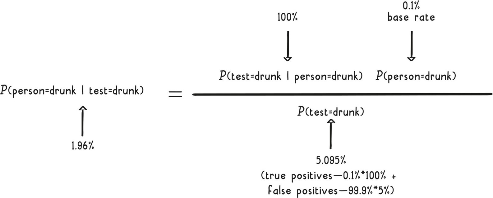
Let’s consider a more realistic base rate, where one in a thousand drivers is drunk, meaning that there is a small chance (0.1 percent) that a person the police randomly pull over is drunk. And since we know one in twenty tests will be wrong (the tests will be wrong 5 percent of the time), the police will most likely go through a lot of wrong tests before they find a person who was actually drunk-driving.

In fact, if the police stop a thousand people, they would on average conduct nearly fifty wrong tests along their way to finding one actual drunk driver. So there is approximately only a 2 percent chance that a failed Breathalyzer in this scenario indicates that the person is actually drunk. Alternatively, this can be stated as a 98 percent chance that the person is sober. That’s way, way more than 5 percent!

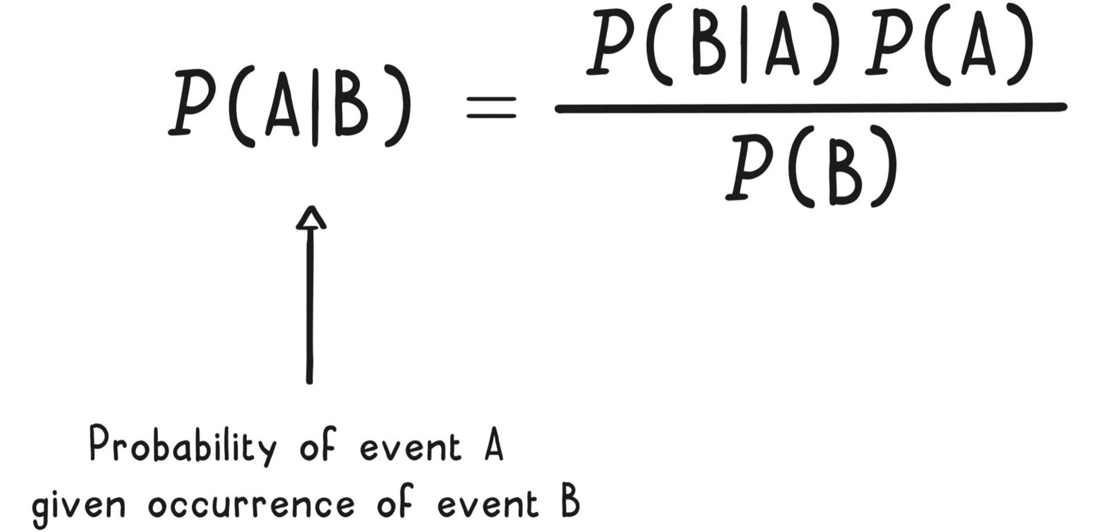
So, P(A|B) does not equal P(B|A), but how are they related? There is a very useful result in probability called Bayes’ theorem, which tells us the relationship between these two conditional probabilities. On the next page, you will see how Bayes’ theorem relates these probabilities and how, in the drunk-driving example, Bayes’ theorem could be applied to calculate the 2 percent result.

Bayes’ Theorem

Base Rate Fallacy

Now that you know about Bayes’ theorem, you should also know that there are two schools of thought in statistics, based on different ways to think about probability: Frequentist and Bayesian. Most studies you hear about in the news are based on frequentist statistics, which relies on and requires many observations of an event before it can make reliable statistical determinations. Frequentists view probability as fundamentally tied to the frequency of events.

By observing the frequency of results over a large sample (e.g., asking a large number of people if they approve of Congress), frequentists estimate an unknown quantity. If there are very few data points, however, they can’t say much of anything, since the confidence intervals they can calculate will be extremely large. In their view, probability without observations makes no sense.

Bayesians, by contrast, allow probabilistic judgments about any situation, regardless of whether any observations have yet occurred. To do this, Bayesians begin by bringing related evidence to statistical determinations. For example, picking a penny up off the street, you’d probably initially estimate a fifty-fifty chance that it would come up heads if you flipped it, even if you’d never observed a flip of that particular coin before. In Bayesian statistics, you can bring such knowledge of base rates to a problem. In frequentist statistics, you cannot.

Many people find this Bayesian way of looking at probability more intuitive because it is similar to how your beliefs naturally evolve. In everyday life, you aren’t starting from scratch every time, as you would in frequentist statistics. For instance, on policy issues, your starting point is what you currently know on that topic—what Bayesians call a prior— and then when you get new data, you (hopefully) update your prior based on the new information. The same is true for relationships, with your starting point being your previous experiences with that person; a strong prior would be a lifelong relationship, whereas a weak prior would be just a first impression.

You saw in the last section that frequentist statistics produce confidence intervals. These statistics tell you that if you ran an experiment many times (e.g., the one-hundred-coin-flips example we presented), the confidence intervals calculated should contain the parameter you are studying (e.g., 50 percent probability of getting heads) to the level of confidence specified (e.g., 95 percent of the time). To many people’s dismay, a confidence interval does not say there is a 95 percent chance of the true value of the parameter being in the interval. By contrast, Bayesian statistics analogously produces credible intervals, which do say that; credible intervals specify the current best estimated range for the probability of the parameter. As such, this Bayesian way of doing things is again more intuitive.

In practice, though, both approaches yield very similar conclusions, and as more data becomes available, they should converge on the same conclusion. That’s because they are both trying to estimate the same underlying truth. Historically, the frequentist viewpoint has been more popular, in large part because Bayesian analysis is often computationally challenging. However, modern computing power is quickly reducing this challenge.

Bayesians contend that by choosing a strong prior, they can start closer to the truth, allowing them to converge on the final result faster, with fewer observations. As observations are expensive in both time and money, this reduction can be attractive. However, there is a flip side: it is also possible that Bayesians’ prior beliefs are actually doing the opposite, starting them further from the truth. This can happen if they have a strong belief that is based on confirmation bias (see Chapter 1) or another cognitive mistake (e.g., an unjustified strong prior). In this case, the Bayesian approach may take longer to converge on the truth because the frequentist view (starting from scratch) is actually closer to the truth at the start.

The takeaway is that two ways of approaching statistics exist, and you should be aware that, done right, both approaches are valid. Some people are hard-core ideologues who pledge allegiance to one philosophy versus the other, whereas pragmatists (like us) use whichever methodology works best for the situation. And more commonly, remember not to confuse a conditional probability with its inverse: P(A|B) is not equal to P(B|A). You now know that these probabilities are related by Bayes’ theorem, which takes into account relevant base rates.

RIGHT OR WRONG?

So far you have learned that you shouldn’t base your decisions on anecdotes and that small samples cannot reliably tell you what will happen in larger populations. You might be wondering, then: How much data is enough data to be sure of my conclusions? Deciding the sample size, the total number of data points collected, is a balancing act. On one side, the more information you collect, the better your estimates will be, and the more sure you can be of your conclusions. On the other side is the fact that gathering more data takes more time and more money, and potentially puts more participants at risk. So, how do you know what the right sample size is? That’s what we cover in this section.

Even with the best experimental design, sometimes you get a fluke result that leads you to draw the wrong conclusions. A higher sample size will give you more confidence that a positive result is not just a fluke and will also give you a greater chance of detecting a positive result.

Consider a typical polling situation, such as measuring public support for an upcoming referendum, e.g., marijuana legalization. Suppose that the referendum ultimately fails, but the pollsters had randomly selected as their respondents people who were more in favor of it when compared with the whole population. This situation could result in a false positive: falsely giving a positive result when it really wasn’t true (like the wrong Breathalyzer test). Conversely, suppose the referendum ultimately succeeds, but the pollsters had randomly selected people less in favor of it when compared with the whole population. This situation could result in a false negative: falsely giving a negative result when it really was true.

As another example, consider a mammogram, a medical test used in the diagnosis of breast cancer. You might think a test like this has two possible results: positive or negative. But really a mammogram has four possible outcomes, depicted in the following table. The two possible outcomes you immediately think of are when the test is right, the true positive and the true negative; the other two outcomes occur when the test is wrong, the false positive and the false negative.

Possible Test Outcomes Results of mammogram
	Evidence of cancer	No evidence of cancer
Patient has breast cancer	True positive	False negative
Patient does not have breast cancer	False positive	True negative

These error models occur well beyond statistics, in any system where judgments are made. Your email spam filter is a good example. Recently our spam filters flagged an email with photos of our new niece as spam (false positive). And actual spam messages still occasionally make it through our spam filters (false negatives).

Because making each type of error has consequences, systems need to be designed with these consequences in mind. That is, you have to make decisions on the trade-off between the different types of error, recognizing that some errors are inevitable. For instance, the U.S. legal system is supposed to require proof beyond a reasonable doubt for criminal convictions. This is a conscious trade-off favoring false negatives (letting criminals go free) over false positives (wrongly convicting people of crimes).

In statistics, a false positive is also known as a type I error and a false negative is also called a type II error. When designing an experiment, scientists get to decide on the probability of each type of error they are willing to tolerate. The most common false positive rate chosen is 5 percent. (This rate is also denoted by the Greek letter α, alpha, which is equal to 100 minus the confidence level. This is why you typically see people say a confidence level of 95 percent.) That means that, on average, if your hypothesis is false, one in twenty experiments (5 percent) will get a false positive result.

Regardless of the sample size of your experiment, you can always choose the false positive error rate. It doesn’t have to be 5 percent; you could choose 1 percent or even 0.1 percent. The catch is that, for a given sample size, when you do set such a low false positive rate, you increase your false negative error rate, possibly failing to detect a real result. This is where the sample size selection comes in.

Once you set your false positive rate, you then determine what sample size you need in order to detect a real result with a high enough probability. This value, called the power of the experiment, is typically selected to be an 80 to 90 percent chance of detection, with a corresponding false negative error rate of 10 to 20 percent. (This rate is also denoted by the Greek letter β, beta, which is equal to 100 minus the power.) Researchers say their study is powered at 80 percent.

Statistical Testing
	Nothing to detect	Something to detect
Detected effect	False positive rate (%) aka type 1 error rate, alpha (α) or significance level Typical rate: 5%	Power (%) 100 - false negative rate Typical level: 80%-90%
Did not detect effect	Confidence level (%) 100 - false positive rate Typical level: 95%	False negative rate (%) aka type II error rate or beta (β) Typical rate: 10%-20%

Let’s consider an example to illustrate how all these models work together. Suppose a company wants to prove that its new sleep meditation app is working. Their background research shows that half of the time, the average person falls asleep within ten minutes. The app developers think that their app can improve this rate, helping more people fall asleep in less than ten minutes.

The developers plan a study in a sleep lab to test their theory. The test group will use their app and the control group will just go to sleep without it. (A real study might have a slightly more complicated design, but this simple design will let us better explain the statistical models.) The statistical setup behind most experiments (including this one) starts with a hypothesis that there is no difference between the groups, called the null hypothesis. If the developers collect sufficient evidence to reject this hypothesis, then they will conclude that their app really does help people fall asleep faster.

That is, the app developers plan to observe both groups and then calculate the percentage of people who fall asleep within ten minutes for each group. If they see enough of a difference between the two percentages, they will conclude that the results are not compatible with the null hypothesis, which would mean their app is likely really working.

The developers also need to specify an alternative hypothesis, which describes the smallest meaningful change they think could occur between the two groups, e.g., 15 percent more people will fall asleep within ten minutes. This is the real result they want their study to confirm and have an 80 percent chance to detect (corresponding to a false negative rate of 20 percent).

This alternative hypothesis is needed to determine the sample size. The smaller the difference in the alternative hypothesis, the more people will be needed to detect it. With the experimental setup described, a sample size of 268 participants is required.

All of these models come together visually in the figure on the next page.

First, look at the bell curves. (Due to the central limit theorem, we can assume that our differences will be approximately normally distributed.) The curve on the left is for the results under the null hypothesis: that there is no real difference between the two groups. That’s why this left bell curve is centered on 0 percent. Even so, some of the time they’d measure a higher or lower difference than zero due to random chance, with larger differences being less likely. That is, due to the underlying variability, even if the app has no real effect, they might still measure differences between the two groups because of the variable times it takes for people to fall asleep.

The other bell curve (on the right) represents the alternative hypothesis that the app developers hope to be true: that there is a 15 percent increase in the percentage of people who fall asleep within ten minutes using the app as compared with people not using the app. Again, even if this hypothesis were true, due to variability, some of the time they’d still measure less than a 15 percent increase, and some of the time more than a 15 percent increase. That’s why the right bell curve is centered on 15 percent.

Statistical Significance

Alpha: 5% Beta: 20% Sample size: 268

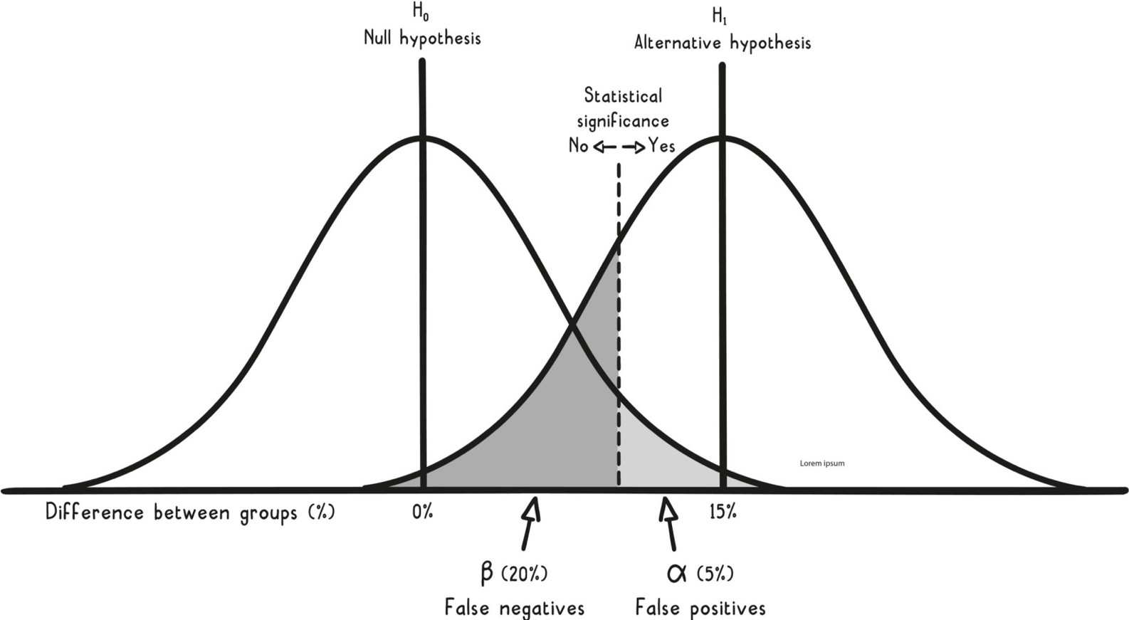
The dotted line represents the threshold for statistical significance. All values larger than this threshold (to the right) would result in rejection of the null hypothesis because differences this large are very unlikely to have occurred if the null hypothesis were true. In fact, they would occur with less than a 5 percent chance—the false positive rate initially set by the developers.

The final measure commonly used to declare whether a result is statistically significant is called the p-value, which is formally defined as the probability of obtaining a result equal to or more extreme than what was observed, assuming the null hypothesis was true. Essentially, if the p-value is smaller than the selected false positive rate (5 percent), then you would say that the result is statistically significant. P-values are commonly used in study reports to communicate such significance.

For example, a p-value of 0.01 would mean that a difference equal to or larger than the one observed would happen only 1 percent of the time if the app had no effect. This value corresponds to a value on the figure in the extreme tail of the left bell curve and close to the middle of the right bell curve. This placement indicates that the result is more consistent with the alternative hypothesis, that the app has an effect of 15 percent.

Now, notice how these two curves overlap, showing that some differences between the two groups are consistent with both hypotheses (under both bell curves simultaneously). These gray areas show where the two types of error can occur. The light gray area is the false positive region and the dark gray area is the false negative region.

A false positive would occur when a large difference is measured between the two groups (like one with a p-value of 0.01), but in reality, the app does nothing. This could happen if the no-app group randomly had trouble falling asleep and the app group randomly had an easy time.

Alternatively, a false negative would occur when the app really does help people fall asleep faster, but the difference observed is too small to be statistically significant. If the study is 80 percent powered, which is typical, this false negative scenario would occur 20 percent of the time.

Assuming the sample size remains fixed, lowering the chance of making a false positive error is equivalent to moving the dotted line to the right, shrinking the light gray area. When you do so, though, the chance of making a false negative error grows (depicted in the following figure as compared with the original).

Statistical Significance

Alpha: 2% Beta: 33% Sample size: 268

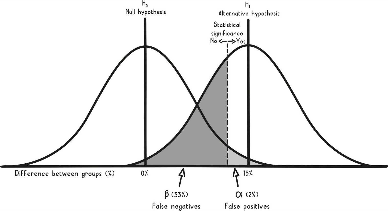
If you want to reduce one of the error rates without increasing the other, you need to increase the sample size. When that happens, each of the bell curves becomes narrower (see the figure below, again as compared to the original).

Statistical Significance

Alpha: 5% Beta: 12% Sample size: 344

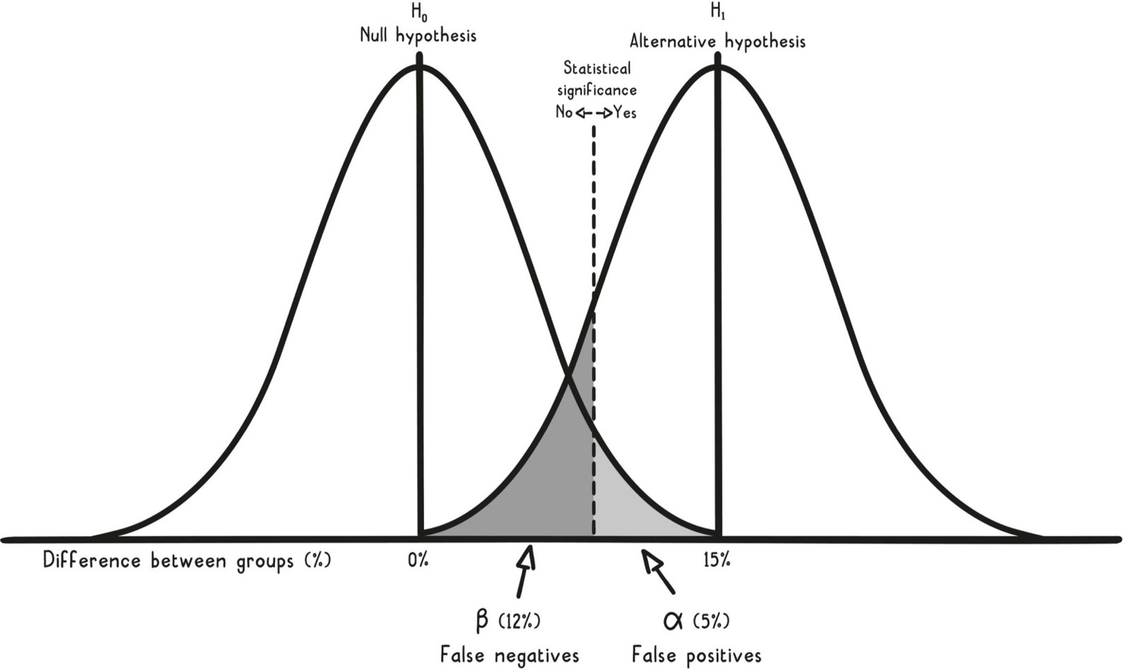
Increasing the sample size and narrowing the bell curves decreases the overlap between the two curves, shrinking the total gray area in the process. This is of course attractive because there is less chance of making an error; however, as we noted in the beginning of this section, there are many reasons why it may not be practical to increase the sample size (time, money, risk to participants, etc.).

The table on the next page illustrates how sample size varies for different limits on the error rates for the sleep app study. You will see that if error rates are decreased, the sample size must be increased.

The sample size values in the following table are all dependent on the selected alternative hypothesis of a 15 percent difference. The sample sizes would all further increase if the developers wanted to detect a smaller difference and would all decrease if they wanted to detect only a larger difference.

Researchers often feel pressure to use a smaller sample size in order to save time and money, which can make choosing a larger difference for the alternative hypothesis appealing. But such a choice comes at a high risk. For instance, the developers can reduce their sample size to just 62 (from 268) if they change the alternative hypothesis to a 30 percent increase between the two groups (up from 15 percent).

Sample Size Varies with Power and Significance
Alpha	Confidence level	Beta	Power	Sample size
10%	90%	20%	80%	196
10%	90%	10%	90%	284
5%	95%	30%	70%	204
5%	95%	20%	80%	268
5%	95%	10%	90%	370
1%	99%	20%	80%	434
1%	99%	10%	90%	562

However, if the true difference the app makes is really only 15 percent, with this smaller sample size they will be able to detect this smaller difference only 32 percent of the time! That’s down from 80 percent originally and means that two-thirds of the time they’d get a false negative, failing to detect the 15 percent difference. As a result, ideally any experiment should be designed to detect the smallest meaningful difference.

One final note on p-values and statistical significance: Most statisticians caution against overreliance on p-values in interpreting the results of a study. Failing to find a significant result (a sufficiently small p-value) is not the same as having confidence that there is no effect. The absence of evidence is not the evidence of absence. Similarly, even though the study may have achieved a low p-value, it might not be a replicable result, which we will explore in the final section.

Statistical significance should not be confused with scientific, human, or economic significance. Even the most minuscule effects can be detected as statistically significant if the sample size is large enough. For example, with enough people in the sleep study, you could potentially detect a 1 percent difference between the two groups, but is that meaningful to any customers? No.

Alternatively, more emphasis could be placed on the difference measured in a study along with its corresponding confidence interval. For the app study, while the customers want to know that they have better chances of falling asleep with the app than without, they also want to know how much better. The developers might even want to increase the sample size in order to be able to guarantee a certain margin of error in their estimates.

Further, the American Statistical Association stressed in The American Statistician in 2016 that “scientific conclusions and business or policy decisions should not be based only on whether a p-value passes a specific threshold.” Focusing too much on the p-value encourages black-and-white thinking and compresses the wealth of information that comes out of a study into just one number. Such a singular focus can make you overlook possible suboptimal choices in a study’s design (e.g., sample size) or biases that could have crept in (e.g., selection bias).

WILL IT REPLICATE?

By now you should know that some experimental results are just flukes. In order to be sure a study result isn’t a fluke, it needs to be replicated. Interestingly, in some fields, such as psychology, there has been a concerted effort to replicate positive results, but those efforts have found that fewer than 50 percent of positive results can be replicated.

That rate is low, and this problem is aptly positive results the replication crisis. This final section offers some models to explain how this happens, and how you can nevertheless gain more confidence in a research area.

Replication efforts are an attempt to distinguish between false positive and true positive results. Consider the chances of replication in each of these two groups. A false positive is expected to replicate—that is, a second false positive is expected to occur in a repetition of the study—only 5 percent of the time. On the other hand, a true positive is expected to replicate 80 to 90 percent of the time, depending on the power of the replication study. For the sake of argument, let’s assume this is 80 percent as we did in the last section.

Using those numbers, a replication rate of 50 percent requires about 60 percent of the studies to have been true positives and 40 percent of them to have been false positives. To see this, consider 100 studies: If 60 were true positives, we would expect 48 of those to replicate (80 percent of 60). Of the remaining 40 false positives, 2 would replicate (5 percent of 40) for a total of 50. The replication rate would then be 50 per 100 studies, or 50 percent.