Predicting the Future

Predicting the Future

All human knowledge is uncertain, inexact, and partial.

—BERTRAND RUSSELL

The sun’ll come out tomorrow. You can bet your bottom dollar there’ll be sun.

—ANNIE

In 1969, before embarking on a doctorate in astrophysics at Princeton, J. Richard Gott III took a trip to Europe. There he saw the Berlin Wall, which had been built eight years earlier. Standing in the shadow of the wall, a stark symbol of the Cold War, he began to wonder how much longer it would continue to divide the East and West.

On the face of it, there’s something absurd about trying to make this kind of prediction. Even setting aside the impossibility of forecasting geopolitics, the question seems mathematically laughable: it’s trying to make a prediction from a single data point.

But as ridiculous as this might seem on its face, we make such predictions all the time, by necessity. You arrive at a bus stop in a foreign city and learn, perhaps, that the other tourist standing there has been waiting seven minutes. When is the next bus likely to arrive? Is it worthwhile to wait—and if so, how long should you do so before giving up?

Or perhaps a friend of yours has been dating somebody for a month and wants your advice: is it too soon to invite them along to an upcoming family wedding? The relationship is off to a good start—but how far ahead is it safe to make plans?

A famous presentation made by Peter Norvig, Google’s director of research, carried the title “The Unreasonable Effectiveness of Data” and enthused about “how billions of trivial data points can lead to understanding.” The media constantly tell us that we’re living in an “age of big data,” when computers can sift through those billions of data points and find patterns invisible to the naked eye. But often the problems most germane to daily human life are at the opposite extreme. Our days are full of “small data.” In fact, like Gott standing at the Berlin Wall, we often have to make an inference from the smallest amount of data we could possibly have: a single observation.

So how do we do it? And how should we?

The story begins in eighteenth-century England, in a domain of inquiry irresistible to great mathematical minds of the time, even those of the clergy: gambling.

Reasoning Backward with the Reverend Bayes

If we be, therefore, engaged by arguments to put trust in past experience, and make it the standard of our future judgement, these arguments must be probable only.

—DAVID HUME

More than 250 years ago, the question of making predictions from small data weighed heavily on the mind of the Reverend Thomas Bayes, a Presbyterian minister in the charming spa town of Tunbridge Wells, England.

If we buy ten tickets for a new and unfamiliar raffle, Bayes imagined, and five of them win prizes, then it seems relatively easy to estimate the raffle’s chances of a win: 5/10, or 50%. But what if instead we buy a single ticket and it wins a prize? Do we really imagine the probability of winning to be 1/1, or 100%? That seems too optimistic. Is it? And if so, by how much? What should we actually guess?

For somebody who has had such an impact on the history of reasoning under uncertainty, Bayes’s own history remains ironically uncertain. He was born in 1701, or perhaps 1702, in the English county of Hertfordshire, or maybe it was London. And in either 1746, ’47, ’48, or ’49 he would write one of the most influential papers in all of mathematics, abandon it unpublished, and move on to other things.

Between those two events we have a bit more certainty. The son of a minister, Bayes went to the University of Edinburgh to study theology, and was ordained like his father. He had mathematical as well as theological interests, and in 1736 he wrote an impassioned defense of Newton’s newfangled “calculus” in response to an attack by Bishop George Berkeley. This work resulted in his election in 1742 as a Fellow of the Royal Society, to whom he was recommended as “a Gentleman … well skilled in Geometry and all parts of Mathematical and Philosophical Learning.”

After Bayes died in 1761, his friend Richard Price was asked to review his mathematical papers to see if they contained any publishable material. Price came upon one essay in particular that excited him—one he said “has great merit, and deserves to be preserved.” The essay concerned exactly the kind of raffle problem under discussion:

Let us then imagine a person present at the drawing of a lottery, who knows nothing of its scheme or of the proportion of Blanks to Prizes in it. Let it further be supposed, that he is obliged to infer this from the number of blanks he hears drawn compared with the number of prizes; and that it is enquired what conclusions in these circumstances he may reasonably make.

Bayes’s critical insight was that trying to use the winning and losing tickets we see to figure out the overall ticket pool that they came from is essentially reasoning backward. And to do that, he argued, we need to first reason forward from hypotheticals. In other words, we need to first determine how probable it is that we would have drawn the tickets we did if various scenarios were true. This probability—known to modern statisticians as the “likelihood”—gives us the information we need to solve the problem.

For instance, imagine we bought three tickets and all three were winners. Now, if the raffle was of the particularly generous sort where all the tickets are winners, then our three-for-three experience would of course happen all of the time; it has a 100% chance in that scenario. If, instead, only half of the raffle’s tickets were winners, our three-for-three experience would happen 1⁄2 × 1⁄2 × 1⁄2 of the time, or in other words 1⁄8 of the time. And if the raffle rewarded only one ticket in a thousand, our outcome would have been incredibly unlikely: 1⁄1,000 × 1⁄1,000 × 1⁄1,000, or one in a billion.

Bayes argued that we should accordingly judge it to be more probable that all the raffle tickets are winners than that half of them are, and in turn more probable that half of them are than that only one in a thousand is. Perhaps we had already intuited as much, but Bayes’s logic offers us the ability to quantify that intuition. All things being equal, we should imagine it to be exactly eight times likelier that all the tickets are winners than that half of them are—because the tickets we drew are exactly eight times likelier (100% versus one-in-eight) in that scenario. Likewise, it’s exactly 125 million times likelier that half the raffle tickets are winners than that there’s only one winning ticket per thousand, which we know by comparing one-in-eight to one-in-a-billion.

This is the crux of Bayes’s argument. Reasoning forward from hypothetical pasts lays the foundation for us to then work backward to the most probable one.

It was an ingenious and innovative approach, but it did not manage to provide a full answer to the raffle problem. In presenting Bayes’s results to the Royal Society, Price was able to establish that if you buy a single raffle ticket and it’s a winner, then there’s a 75% chance that at least half the tickets are winners. But thinking about the probabilities of probabilities can get a bit head-spinning. What’s more, if someone pressed us, “Well, fine, but what do you think the raffle odds actually are?” we still wouldn’t know what to say.

The answer to this question—how to distill all the various possible hypotheses into a single specific expectation—would be discovered only a few years later, by the French mathematician Pierre-Simon Laplace.

Laplace’s Law

Laplace was born in Normandy in 1749, and his father sent him to a Catholic school with the intent that he join the clergy. Laplace went on to study theology at the University of Caen, but unlike Bayes—who balanced spiritual and scientific devotions his whole life—he ultimately abandoned the cloth entirely for mathematics.

In 1774, completely unaware of the previous work by Bayes, Laplace published an ambitious paper called “Treatise on the Probability of the Causes of Events.” In it, Laplace finally solved the problem of how to make inferences backward from observed effects to their probable causes.

Bayes, as we saw, had found a way to compare the relative probability of one hypothesis to another. But in the case of a raffle, there is literally an infinite number of hypotheses: one for every conceivable proportion of winning tickets. Using calculus, the once-controversial mathematics of which Bayes had been an important defender, Laplace was able to prove that this vast spectrum of possibilities could be distilled down to a single estimate, and a stunningly concise one at that. If we really know nothing about our raffle ahead of time, he showed, then after drawing a winning ticket on our first try we should expect that the proportion of winning tickets in the whole pool is exactly 2/3. If we buy three tickets and all of them are winners, the expected proportion of winning tickets is exactly 4/5. In fact, for any possible drawing of w winning tickets in n attempts, the expectation is simply the number of wins plus one, divided by the number of attempts plus two: (w+1)⁄(n+2).

This incredibly simple scheme for estimating probabilities is known as Laplace’s Law, and it is easy to apply in any situation where you need to assess the chances of an event based on its history. If you make ten attempts at something and five of them succeed, Laplace’s Law estimates your overall chances to be 6/12 or 50%, consistent with our intuitions. If you try only once and it works out, Laplace’s estimate of 2/3 is both more reasonable than assuming you’ll win every time, and more actionable than Price’s guidance (which would tell us that there is a 75% metaprobability of a 50% or greater chance of success).

Laplace went on to apply his statistical approach to a wide range of problems of his time, including assessing whether babies are truly equally likely to be born male or female. (He established, to a virtual certainty, that male infants are in fact slightly more likely than female ones.) He also wrote the Philosophical Essay on Probabilities, arguably the first book about probability for a general audience and still one of the best, laying out his theory and considering its applications to law, the sciences, and everyday life.

Laplace’s Law offers us the first simple rule of thumb for confronting small data in the real world. Even when we’ve made only a few observations—or only one—it offers us practical guidance. Want to calculate the chance your bus is late? The chance your softball team will win? Count the number of times it has happened in the past plus one, then divide by the number of opportunities plus two. And the beauty of Laplace’s Law is that it works equally well whether we have a single data point or millions of them. Little Annie’s faith that the sun will rise tomorrow is justified, it tells us: with an Earth that’s seen the sun rise for about 1.6 trillion days in a row, the chance of another sunrise on the next “attempt” is all but indistinguishable from 100%.

Bayes’s Rule and Prior Beliefs

All these suppositions are consistent and conceivable. Why should we give the preference to one, which is no more consistent or conceivable than the rest?

—DAVID HUME

Laplace also considered another modification to Bayes’s argument that would prove crucial: how to handle hypotheses that are simply more probable than others. For instance, while it’s possible that a lottery might give away prizes to 99% of the people who buy tickets, it’s more likely—we’d assume—that they would give away prizes to only 1%. That assumption should be reflected in our estimates.

To make things concrete, let’s say a friend shows you two different coins. One is a normal, “fair” coin with a 50–50 chance of heads and tails; the other is a two-headed coin. He drops them into a bag and then pulls one out at random. He flips it once: heads. Which coin do you think your friend flipped?

Bayes’s scheme of working backward makes short work of this question. A flip coming up heads happens 50% of the time with a fair coin and 100% of the time with a two-headed coin. Thus we can assert confidently that it’s 100%⁄50%, or exactly twice as probable, that the friend had pulled out the two-headed coin.

Now consider the following twist. This time, the friend shows you nine fair coins and one two-headed coin, puts all ten into a bag, draws one at random, and flips it: heads. Now what do you suppose? Is it a fair coin or the two-headed one?

Laplace’s work anticipated this wrinkle, and here again the answer is impressively simple. As before, a fair coin is exactly half as likely to come up heads as a two-headed coin. But now, a fair coin is also nine times as likely to have been drawn in the first place. It turns out that we can just take these two different considerations and multiply them together: it is exactly four and a half times more likely that your friend is holding a fair coin than the two-headed one.

The mathematical formula that describes this relationship, tying together our previously held ideas and the evidence before our eyes, has come to be known—ironically, as the real heavy lifting was done by Laplace—as Bayes’s Rule. And it gives a remarkably straightforward solution to the problem of how to combine preexisting beliefs with observed evidence: multiply their probabilities together.

Notably, having some preexisting beliefs is crucial for this formula to work. If your friend simply approached you and said, “I flipped one coin from this bag and it came up heads. How likely do you think it is that this is a fair coin?,” you would be totally unable to answer that question unless you had at least some sense of what coins were in the bag to begin with. (You can’t multiply the two probabilities together when you don’t have one of them.) This sense of what was “in the bag” before the coin flip—the chances for each hypothesis to have been true before you saw any data—is known as the prior probabilities, or “prior” for short. And Bayes’s Rule always needs some prior from you, even if it’s only a guess. How many two-headed coins exist? How easy are they to get? How much of a trickster is your friend, anyway?

The fact that Bayes’s Rule is dependent on the use of priors has at certain points in history been considered controversial, biased, even unscientific. But in reality, it is quite rare to go into a situation so totally unfamiliar that our mind is effectively a blank slate—a point we’ll return to momentarily.

When you do have some estimate of prior probabilities, meanwhile, Bayes’s Rule applies to a wide range of prediction problems, be they of the big-data variety or the more common small-data sort. Computing the probability of winning a raffle or tossing heads is only the beginning. The methods developed by Bayes and Laplace can offer help any time you have uncertainty and a bit of data to work with. And that’s exactly the situation we face when we try to predict the future.

The Copernican Principle

It’s difficult to make predictions, especially about the future.

—DANISH PROVERB

When J. Richard Gott arrived at the Berlin Wall, he asked himself a very simple question: Where am I? That is to say, where in the total life span of this artifact have I happened to arrive? In a way, he was asking the temporal version of the spatial question that had obsessed the astronomer Nicolaus Copernicus four hundred years earlier: Where are we? Where in the universe is the Earth? Copernicus would make the radical paradigm shift of imagining that the Earth was not the bull’s-eye center of the universe—that it was, in fact, nowhere special in particular. Gott decided to take the same step with regard to time.

He made the assumption that the moment when he encountered the Berlin Wall wasn’t special—that it was equally likely to be any moment in the wall’s total lifetime. And if any moment was equally likely, then on average his arrival should have come precisely at the halfway point (since it was 50% likely to fall before halfway and 50% likely to fall after). More generally, unless we know better we can expect to have shown up precisely halfway into the duration of any given phenomenon.* And if we assume that we’re arriving precisely halfway into something’s duration, the best guess we can make for how long it will last into the future becomes obvious: exactly as long as it’s lasted already. Gott saw the Berlin Wall eight years after it was built, so his best guess was that it would stand for eight years more. (It ended up being twenty.)

This straightforward reasoning, which Gott named the Copernican Principle, results in a simple algorithm that can be used to make predictions about all sorts of topics. Without any preconceived expectations, we might use it to obtain predictions for the end of not only the Berlin Wall but any number of other short- and long-lived phenomena. The Copernican Principle predicts that the United States of America will last as a nation until approximately the year 2255, that Google will last until roughly 2032, and that the relationship your friend began a month ago will probably last about another month (maybe tell him not to RSVP to that wedding invitation just yet). Likewise, it tells us to be skeptical when, for instance, a recent New Yorker cover depicts a man holding a six-inch smartphone with a familiar grid of square app icons, and the caption reads “2525.” Doubtful. The smartphone as we know it is barely a decade old, and the Copernican Principle tells us that it isn’t likely to be around in 2025, let alone five centuries later. By 2525 it’d be mildly surprising if there were even a New York City.

More practically, if we’re considering employment at a construction site whose signage indicates that it’s been “7 days since the last industrial accident,” we might want to stay away, unless it’s a particularly short job we plan to do. And if a municipal transit system cannot afford the incredibly useful but expensive real-time signs that tell riders when the next bus is going to arrive, the Copernican Principle suggests that there might be a dramatically simpler and cheaper alternative. Simply displaying how long it’s been since the previous bus arrived at that stop offers a substantial hint about when the next one will.

But is the Copernican Principle right? After Gott published his conjecture in Nature, the journal received a flurry of critical correspondence. And it’s easy to see why when we try to apply the rule to some more familiar examples. If you meet a 90-year-old man, the Copernican Principle predicts he will live to 180. Every 6-year-old boy, meanwhile, is predicted to face an early death at the tender age of 12.

To understand why the Copernican Principle works, and why it sometimes doesn’t, we need to return to Bayes. Because despite its apparent simplicity, the Copernican Principle is really an instance of Bayes’s Rule.

Bayes Meets Copernicus

When predicting the future, such as the longevity of the Berlin Wall, the hypotheses we need to evaluate are all the possible durations of the phenomenon at hand: will it last a week, a month, a year, a decade? To apply Bayes’s Rule, as we have seen, we first need to assign a prior probability to each of these durations. And it turns out that the Copernican Principle is exactly what results from applying Bayes’s Rule using what is known as an uninformative prior.

At first this may seem like a contradiction in terms. If Bayes’s Rule always requires us to specify our prior expectations and beliefs, how could we tell it that we don’t have any? In the case of a raffle, one way to plead ignorance would be to assume what’s called the “uniform prior,” which considers every proportion of winning tickets to be equally likely.* In the case of the Berlin Wall, an uninformative prior means saying that we don’t know anything about the time span we’re trying to predict: the wall could equally well come down in the next five minutes or last for five millennia.

Aside from that uninformative prior, the only piece of data we supply to Bayes’s Rule, as we’ve seen, is the fact that we’ve encountered the Berlin Wall when it is eight years old. Any hypothesis that would have predicted a less than eight-year life span for the wall is thereby ruled out immediately, since those hypotheses can’t account for our situation at all. (Similarly, a two-headed coin is ruled out by the first appearance of tails.) Anything longer than eight years is within the realm of possibility—but if the wall were going to be around for a million years, it would be a big coincidence that we happened to bump into it so very close to the start of its existence. Therefore, even though enormously long life spans cannot be ruled out, neither are they very likely.

When Bayes’s Rule combines all these probabilities—the more-probable short time spans pushing down the average forecast, the less-probable yet still possible long ones pushing it up—the Copernican Principle emerges: if we want to predict how long something will last, and have no other knowledge about it whatsoever, the best guess we can make is that it will continue just as long as it’s gone on so far.

In fact, Gott wasn’t even the first to propose something like the Copernican Principle. In the mid-twentieth century, the Bayesian statistician Harold Jeffreys had looked into determining the number of tramcars in a city given the serial number on just one tramcar, and came up with the same answer: double the serial number. And a similar problem had arisen even earlier, during World War II, when the Allies sought to estimate the number of tanks being produced by Germany. Purely mathematical estimates based on captured tanks’ serial numbers predicted that the Germans were producing 246 tanks every month, while estimates obtained by extensive (and highly risky) aerial reconnaissance suggested the figure was more like 1,400. After the war, German records revealed the true figure: 245.

Recognizing that the Copernican Principle is just Bayes’s Rule with an uninformative prior answers a lot of questions about its validity. The Copernican Principle seems reasonable exactly in those situations where we know nothing at all—such as looking at the Berlin Wall in 1969, when we’re not even sure what timescale is appropriate. And it feels completely wrong in those cases where we do know something about the subject matter. Predicting that a 90-year-old man will live to 180 years seems unreasonable precisely because we go into the problem already knowing a lot about human life spans—and so we can do better. The richer the prior information we bring to Bayes’s Rule, the more useful the predictions we can get out of it.

Real-World Priors …

In the broadest sense, there are two types of things in the world: things that tend toward (or cluster around) some kind of “natural” value, and things that don’t.

Human life spans are clearly in the former category. They roughly follow what’s termed a “normal” distribution—also known as the “Gaussian” distribution, after the German mathematician Carl Friedrich Gauss, and informally called the “bell curve” for its characteristic shape. This shape does a good job of characterizing human life spans; the average life span for men in the United States, for instance, is centered at about 76 years, and the probabilities fall off fairly sharply to either side. Normal distributions tend to have a single appropriate scale: a one-digit life span is considered tragic, a three-digit one extraordinary. Many other things in the natural world are normally distributed as well, from human height, weight, and blood pressure to the noontime temperature in a city and the diameter of fruits in an orchard.

There are a number of things in the world that don’t look normally distributed, however—not by a long shot. The average population of a town in the United States, for instance, is 8,226. But if you were to make a graph of the number of towns by population, you wouldn’t see anything remotely like a bell curve. There would be way more towns smaller than 8,226 than larger. At the same time, the larger ones would be way bigger than the average. This kind of pattern typifies what are called “power-law distributions.” These are also known as “scale-free distributions” because they characterize quantities that can plausibly range over many scales: a town can have tens, hundreds, thousands, tens of thousands, hundreds of thousands, or millions of residents, so we can’t pin down a single value for how big a “normal” town should be.

The power-law distribution characterizes a host of phenomena in everyday life that have the same basic quality as town populations: most things below the mean, and a few enormous ones above it. Movie box-office grosses, which can range from four to ten figures, are another example. Most movies don’t make much money at all, but the occasional Titanic makes … well, titanic amounts.

In fact, money in general is a domain full of power laws. Power-law distributions characterize both people’s wealth and people’s incomes. The mean income in America, for instance, is $55,688—but because income is roughly power-law distributed, we know, again, that many more people will be below this mean than above it, while those who are above might be practically off the charts. So it is: two-thirds of the US population make less than the mean income, but the top 1% make almost ten times the mean. And the top 1% of the 1% make ten times more than that.

It’s often lamented that “the rich get richer,” and indeed the process of “preferential attachment” is one of the surest ways to produce a power-law distribution. The most popular websites are the most likely to get incoming links; the most followed online celebrities are the ones most likely to gain new fans; the most prestigious firms are the ones most likely to attract new clients; the biggest cities are the ones most likely to draw new residents. In every case, a power-law distribution will result.

Bayes’s Rule tells us that when it comes to making predictions based on limited evidence, few things are as important as having good priors—that is, a sense of the distribution from which we expect that evidence to have come. Good predictions thus begin with having good instincts about when we’re dealing with a normal distribution and when with a power-law distribution. As it turns out, Bayes’s Rule offers us a simple but dramatically different predictive rule of thumb for each.

… and Their Prediction Rules

Did you mean “this could go on forever” in a good way?

—BEN LERNER

Examining the Copernican Principle, we saw that when Bayes’s Rule is given an uninformative prior, it always predicts that the total life span of an object will be exactly double its current age. In fact, the uninformative prior, with its wildly varying possible scales—the wall that might last for months or for millennia—is a power-law distribution. And for any power-law distribution, Bayes’s Rule indicates that the appropriate prediction strategy is a Multiplicative Rule: multiply the quantity observed so far by some constant factor. For an uninformative prior, that constant factor happens to be 2, hence the Copernican prediction; in other power-law cases, the multiplier will depend on the exact distribution you’re working with. For the grosses of movies, for instance, it happens to be about 1.4. So if you hear a movie has made $6 million so far, you can guess it will make about $8.4 million overall; if it’s made $90 million, guess it will top out at $126 million.

This multiplicative rule is a direct consequence of the fact that power-law distributions do not specify a natural scale for the phenomenon they’re describing. The only thing that gives us a sense of scale for our prediction, therefore, is the single data point we have—such as the fact that the Berlin Wall has stood for eight years. The larger the value of that single data point, the larger the scale we’re probably dealing with, and vice versa. It’s possible that a movie that’s grossed $6 million is actually a blockbuster in its first hour of release, but it’s far more likely to be just a single-digit-millions kind of movie.

When we apply Bayes’s Rule with a normal distribution as a prior, on the other hand, we obtain a very different kind of guidance. Instead of a multiplicative rule, we get an Average Rule: use the distribution’s “natural” average—its single, specific scale—as your guide. For instance, if somebody is younger than the average life span, then simply predict the average; as their age gets close to and then exceeds the average, predict that they’ll live a few years more. Following this rule gives reasonable predictions for the 90-year-old and the 6-year-old: 94 and 77, respectively. (The 6-year-old gets a tiny edge over the population average of 76 by virtue of having made it through infancy: we know he’s not in the distribution’s left tail.)

Movie running times, like human lifetimes, also follow a normal distribution: most films cluster right around a hundred minutes or so, with diminishing numbers of exceptions tailing off to either side. But not all human activities are so well behaved. The poet Dean Young once remarked that whenever he’s listening to a poem in numbered sections, his heart sinks if the reader announces the start of section four: if there are more than three parts, all bets are off, and Young needs to hunker down for an earful. It turns out that Young’s dismay is, in fact, perfectly Bayesian. An analysis of poems shows that, unlike movie running times, poems follow something closer to a power-law than a normal distribution: most poems are short, but some are epics. So when it comes to poetry, make sure you’ve got a comfortable seat. Something normally distributed that’s gone on seemingly too long is bound to end shortly; but the longer something in a power-law distribution has gone on, the longer you can expect it to keep going.

Between those two extremes, there’s actually a third category of things in life: those that are neither more nor less likely to end just because they’ve gone on for a while. Sometimes things are simply … invariant. The Danish mathematician Agner Krarup Erlang, who studied such phenomena, formalized the spread of intervals between independent events into the function that now carries his name: the Erlang distribution. The shape of this curve differs from both the normal and the power-law: it has a winglike contour, rising to a gentle hump, with a tail that falls off faster than a power-law but more slowly than a normal distribution. Erlang himself, working for the Copenhagen Telephone Company in the early twentieth century, used it to model how much time could be expected to pass between successive calls on a phone network. Since then, the Erlang distribution has also been used by urban planners and architects to model car and pedestrian traffic, and by networking engineers designing infrastructure for the Internet. There are a number of domains in the natural world, too, where events are completely independent from one another and the intervals between them thus fall on an Erlang curve. Radioactive decay is one example, which means that the Erlang distribution perfectly models when to expect the next ticks of a Geiger counter. It also turns out to do a pretty good job of describing certain human endeavors—such as the amount of time politicians stay in the House of Representatives.

The Erlang distribution gives us a third kind of prediction rule, the Additive Rule: always predict that things will go on just a constant amount longer. The familiar refrain of “Just five more minutes!… [five minutes later] Five more minutes!” that so often characterizes human claims regarding, say, one’s readiness to leave the house or office, or the time until the completion of some task, may seem indicative of some chronic failure to make realistic estimates. Well, in the cases where one’s up against an Erlang distribution, anyway, that refrain happens to be correct.

If a casino card-playing enthusiast tells his impatient spouse, for example, that he’ll quit for the day after hitting one more blackjack (the odds of which are about 20 to 1), he might cheerily predict, “I’ll be done in about twenty more hands!” If, an unlucky twenty hands later, she returns, asking how long he’s going to make her wait now, his answer will be unchanged: “I’ll be done in about twenty more hands!” It sounds like our indefatigable card shark has suffered a short-term memory loss—but, in fact, his prediction is entirely correct. Indeed, distributions that yield the same prediction, no matter their history or current state, are known to statisticians as “memoryless.”

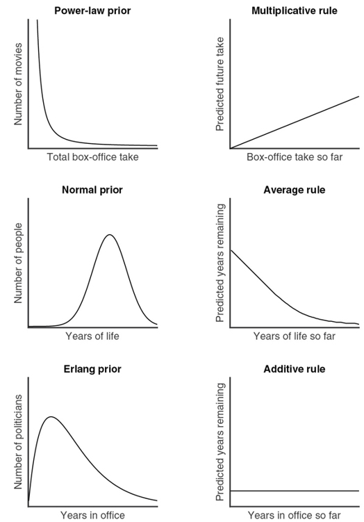
Different prior distributions and their prediction rules.

These three very different patterns of optimal prediction—the Multiplicative, Average, and Additive Rules—all result directly from applying Bayes’s Rule to the power-law, normal, and Erlang distributions, respectively. And given the way those predictions come out, the three distributions offer us different guidance, too, on how surprised we should be by certain events.

In a power-law distribution, the longer something has gone on, the longer we expect it to continue going on. So a power-law event is more surprising the longer we’ve been waiting for it—and maximally surprising right before it happens. A nation, corporation, or institution only grows more venerable with each passing year, so it’s always stunning when it collapses.

In a normal distribution, events are surprising when they’re early—since we expected them to reach the average—but not when they’re late. Indeed, by that point they seem overdue to happen, so the longer we wait, the more we expect them.

And in an Erlang distribution, events by definition are never any more or less surprising no matter when they occur. Any state of affairs is always equally likely to end regardless of how long it’s lasted. No wonder politicians are always thinking about their next election.

Gambling is characterized by a similar kind of steady-state expectancy. If your wait for, say, a win at the roulette wheel were characterized by a normal distribution, then the Average Rule would apply: after a run of bad luck, it’d tell you that your number should be coming any second, probably followed by more losing spins. (In that case, it’d make sense to press on to the next win and then quit.) If, instead, the wait for a win obeyed a power-law distribution, then the Multiplicative Rule would tell you that winning spins follow quickly after one another, but the longer a drought had gone on the longer it would probably continue. (In that scenario, you’d be right to keep playing for a while after any win, but give up after a losing streak.) Up against a memoryless distribution, however, you’re stuck. The Additive Rule tells you the chance of a win now is the same as it was an hour ago, and the same as it will be an hour from now. Nothing ever changes. You’re not rewarded for sticking it out and ending on a high note; neither is there a tipping point when you should just cut your losses. In “The Gambler,” Kenny Rogers famously advised that you’ve got to “Know when to walk away / Know when to run”—but for a memoryless distribution, there is no right time to quit. This may in part explain these games’ addictiveness.

Knowing what distribution you’re up against can make all the difference. When the Harvard biologist and prolific popularizer of science Stephen Jay Gould discovered that he had cancer, his immediate impulse was to read the relevant medical literature. Then he found out why his doctors had discouraged him from doing so: half of all patients with his form of cancer died within eight months of discovery.

But that one statistic—eight months—didn’t tell him anything about the distribution of survivors. If it were a normal distribution, then the Average Rule would give a pretty clear forecast of how long he could expect to live: about eight months. But if it were a power-law, with a tail that stretches far out to the right, then the situation would be quite different: the Multiplicative Rule would tell him that the longer he lived, the more evidence it would provide that he would live longer. Reading further, Gould discovered that “the distribution was indeed, strongly right skewed, with a long tail (however small) that extended for several years above the eight month median. I saw no reason why I shouldn’t be in that small tail, and I breathed a very long sigh of relief.” Gould would go on to live for twenty more years after his diagnosis.

Small Data and the Mind

The three prediction rules—Multiplicative, Average, and Additive—are applicable in a wide range of everyday situations. And in those situations, people in general turn out to be remarkably good at using the right prediction rule. When he was in graduate school, Tom, along with MIT’s Josh Tenenbaum, ran an experiment asking people to make predictions for a variety of everyday quantities—such as human life spans, the grosses of movies, and the time that US representatives would spend in office—based on just one piece of information in each case: current age, money earned so far, and years served to date. Then they compared the predictions people made to the predictions given by applying Bayes’s Rule to the actual real-world data across each of those domains.

As it turned out, the predictions that people had made were extremely close to those produced by Bayes’s Rule. Intuitively, people made different types of predictions for quantities that followed different distributions—power-law, normal, and Erlang—in the real world. In other words, while you might not know or consciously remember which situation calls for the Multiplicative, Average, or Additive Rule, the predictions you make every day tend to implicitly reflect the different cases where these distributions appear in everyday life, and the different ways they behave.

In light of what we know about Bayes’s Rule, this remarkably good human performance suggests something critical that helps to understand how people make predictions. Small data is big data in disguise. The reason we can often make good predictions from a small number of observations—or just a single one—is that our priors are so rich. Whether we know it or not, we appear to carry around in our heads surprisingly accurate priors about movie grosses and running times, poem lengths, and political terms of office, not to mention human life spans. We don’t need to gather them explicitly; we absorb them from the world.

The fact that, on the whole, people’s hunches seem to closely match the predictions of Bayes’s Rule also makes it possible to reverse-engineer all kinds of prior distributions, even ones about which it’s harder to get authoritative real-world data. For instance, being kept on hold by customer service is a lamentably common facet of human experience, but there aren’t publicly available data sets on hold times the way there are for Hollywood box-office grosses. But if people’s predictions are informed by their experiences, we can use Bayes’s Rule to conduct indirect reconnaissance about the world by mining people’s expectations. When Tom and Josh asked people to predict hold times from a single data point, the results suggested that their subjects were using the Multiplicative Rule: the total wait people expect is one and a third times as long as they’ve waited so far. This is consistent with having a power-law distribution as a prior, where a wide range of scales is possible. Just hope you don’t end up on the Titanic of hold times. Over the past decade, approaches like these have enabled cognitive scientists to identify people’s prior distributions across a broad swath of domains, from vision to language.

There’s a crucial caveat here, however. In cases where we don’t have good priors, our predictions aren’t good. In Tom and Josh’s study, for instance, there was one subject where people’s predictions systematically diverged from Bayes’s Rule: predicting the length of the reign of Egyptian pharaohs. (As it happens, pharaohs’ reigns follow an Erlang distribution.) People simply didn’t have enough everyday exposure to have an intuitive feel for the range of those values, so their predictions, of course, faltered. Good predictions require good priors.

This has a number of important implications. Our judgments betray our expectations, and our expectations betray our experience. What we project about the future reveals a lot—about the world we live in, and about our own past.

What Our Predictions Tell Us About Ourselves

When Walter Mischel ran his famous “marshmallow test” in the early 1970s, he was trying to understand how the ability to delay gratification develops with age. At a nursery school on the Stanford campus, a series of three-, four-, and five-year-olds had their willpower tested. Each child would be shown a delicious treat, such as a marshmallow, and told that the adult running the experiment was about to leave the room for a while. If they wanted to, they could eat the treat right away. But if they waited until the experimenter came back, they would get two treats.

Unable to resist, some of the children ate the treat immediately. And some of them stuck it out for the full fifteen minutes or so until the experimenter returned, and got two treats as promised. But perhaps the most interesting group comprised the ones in between—the ones who managed to wait a little while, but then surrendered and ate the treat.

These cases, where children struggled mightily and suffered valiantly, only to give in and lose the extra marshmallow anyway, have been interpreted as suggesting a kind of irrationality. If you’re going to cave, why not just cave immediately, and skip the torture? But it all depends on what kind of situation the children think they are in. As the University of Pennsylvania’s Joe McGuire and Joe Kable have pointed out, if the amount of time it takes for adults to come back is governed by a power-law distribution—with long absences suggesting even longer waits lie ahead—then cutting one’s losses at some point can make perfect sense.

In other words, the ability to resist temptation may be, at least in part, a matter of expectations rather than willpower. If you predict that adults tend to come back after short delays—something like a normal distribution—you should be able to hold out. The Average Rule suggests that after a painful wait, the thing to do is hang in there: the experimenter should be returning any minute now. But if you have no idea of the timescale of the disappearance—consistent with a power-law distribution—then it’s an uphill battle. The Multiplicative Rule then suggests that a protracted wait is just a small fraction of what’s to come.

Decades after the original marshmallow experiments, Walter Mischel and his colleagues went back and looked at how the participants were faring in life. Astonishingly, they found that children who had waited for two treats grew into young adults who were more successful than the others, even measured by quantitative metrics like their SAT scores. If the marshmallow test is about willpower, this is a powerful testament to the impact that learning self-control can have on one’s life. But if the test is less about will than about expectations, then this tells a different, perhaps more poignant story.

A team of researchers at the University of Rochester recently explored how prior experiences might affect behavior in the marshmallow test. Before marshmallows were even mentioned, the kids in the experiment embarked on an art project. The experimenter gave them some mediocre supplies, and promised to be back with better options soon. But, unbeknownst to them, the children were divided into two groups. In one group, the experimenter was reliable, and came back with the better art supplies as promised. In the other, she was unreliable, coming back with nothing but apologies.

The art project completed, the children went on to the standard marshmallow test. And here, the children who had learned that the experimenter was unreliable were more likely to eat the marshmallow before she came back, losing the opportunity to earn a second treat.

Failing the marshmallow test—and being less successful in later life—may not be about lacking willpower. It could be a result of believing that adults are not dependable: that they can’t be trusted to keep their word, that they disappear for intervals of arbitrary length. Learning self-control is important, but it’s equally important to grow up in an environment where adults are consistently present and trustworthy.

Priors in the Age of Mechanical Reproduction

As if someone were to buy several copies of the morning paper to assure himself that what it said was true.

—LUDWIG WITTGENSTEIN

He is careful of what he reads, for that is what he will write. He is careful of what he learns, for that is what he will know.

—ANNIE DILLARD

The best way to make good predictions, as Bayes’s Rule shows us, is to be accurately informed about the things you’re predicting. That’s why we can do a good job of projecting human life spans, but perform poorly when asked to estimate the reigns of pharaohs.

Being a good Bayesian means representing the world in the correct proportions—having good priors, appropriately calibrated. By and large, for humans and other animals this happens naturally; as a rule, when something surprises us, it ought to surprise us, and when it doesn’t, it ought not to. Even when we accumulate biases that aren’t objectively correct, they still usually do a reasonable job of reflecting the specific part of the world we live in. For instance, someone living in a desert climate might overestimate the amount of sand in the world, and someone living at the poles might overestimate the amount of snow. Both are well tuned to their own ecological niche.

Everything starts to break down, however, when a species gains language. What we talk about isn’t what we experience—we speak chiefly of interesting things, and those tend to be things that are uncommon. More or less by definition, events are always experienced at their proper frequencies, but this isn’t at all true of language. Anyone who has experienced a snake bite or a lightning strike will tend to retell those singular stories for the rest of their lives. And those stories will be so salient that they will be picked up and retold by others.

There’s a curious tension, then, between communicating with others and maintaining accurate priors about the world. When people talk about what interests them—and offer stories they think their listeners will find interesting—it skews the statistics of our experience. That makes it hard to maintain appropriate prior distributions. And the challenge has only increased with the development of the printing press, the nightly news, and social media—innovations that allow our species to spread language mechanically.

Consider how many times you’ve seen either a crashed plane or a crashed car. It’s entirely possible you’ve seen roughly as many of each—yet many of those cars were on the road next to you, whereas the planes were probably on another continent, transmitted to you via the Internet or television. In the United States, for instance, the total number of people who have lost their lives in commercial plane crashes since the year 2000 would not be enough to fill Carnegie Hall even half full. In contrast, the number of people in the United States killed in car accidents over that same time is greater than the entire population of Wyoming.

Simply put, the representation of events in the media does not track their frequency in the world. As sociologist Barry Glassner notes, the murder rate in the United States declined by 20% over the course of the 1990s, yet during that time period the presence of gun violence on American news increased by 600%.

If you want to be a good intuitive Bayesian—if you want to naturally make good predictions, without having to think about what kind of prediction rule is appropriate—you need to protect your priors. Counterintuitively, that might mean turning off the news.

• The image illustrates different prior distributions and their corresponding prediction rules.

References

- An Essay towards Solving a Problem in the Doctrine of Chances — Thomas Bayes (1763)
- Treatise on the Probability of the Causes of Events — Pierre-Simon Laplace (1774)
- Implications of the Copernican Principle for Our Future Prospects — J. Richard Gott III (1993)
- Theory of Probability — Harold Jeffreys (1961)
- The Unreasonable Effectiveness of Data — Peter Norvig (2009)
CONTINUE THE CONVERSATION
Source texts
- Algorithms to Live By The Computer Science of Human Decisions (Brian Christian, Tom Griffiths)