Mean Squared Error (MSE) and the Least Squares Method

Mean Squared Error

The original Figure 6, showing mean squared error for ten possible values of the true length, is not included in this excerpt. In that example, overall error increases rapidly as the estimate moves away from the mean. When your estimate increases by just 3 millimeters, from 976 to 979, for instance, MSE doubles. This is a key feature of MSE: squaring gives large errors a far greater weight than it gives small ones.

You now see why Gauss's formula to measure overall error is called mean squared error and why his approach to estimation is called the least squares method. The squaring of errors is its central idea: the mean minimizes the sum of squared deviations.

The advantages of Gauss's approach were quickly recognized by other mathematicians. Among his many feats, Gauss used MSE (and other mathematical innovations) to solve a puzzle that had defeated the best astronomers of Europe: the rediscovery of Ceres, an asteroid that had been traced only briefly before it disappeared into the glare of the sun in 1801. The astronomers had been trying to estimate Ceres's trajectory, but the way they accounted for the measurement error of their telescopes was wrong, and the planet did not reappear anywhere near the location their results suggested. Gauss redid their calculations, using the least squares method. When the astronomers trained their telescopes to the spot that he had indicated, they found Ceres!

Scientists in diverse disciplines were quick to adopt the least squares method. Over two centuries later, it remains the standard way to evaluate errors wherever achieving accuracy is the goal. The weighting of errors by their square is central to statistics. In the vast majority of applications across all scientific disciplines, MSE rules. As we are about to see, the approach has surprising implications.

The Error Equations

The role of bias and noise in error is easily summarized in two expressions that we will call the error equations. The first of these equations decomposes the error in a single measurement into the two components with which you are now familiar: bias—the average error—and a residual "noisy error." The noisy error is positive when the error is larger than the bias, negative when it is smaller. The average of noisy errors is zero. Nothing new in the first error equation.

Error in a single measurement = Bias + Noisy Error

The second error equation is a decomposition of MSE, the measure of overall error we have now introduced. Using some simple algebra, MSE can be shown to be equal to the sum of the squares of bias and noise. (Recall that noise is the standard deviation of measurements, which is identical to the standard deviation of noisy errors.) Therefore:

Overall Error (MSE) = Bias^2 + Noise^2

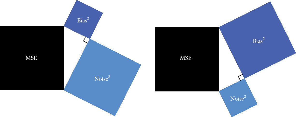
The form of this equation—a sum of two squares—may remind you of a high-school favorite, the Pythagorean theorem. As you might remember, in a right triangle, the sum of the squares of the two shorter sides equals the square of the longest one. This suggests a simple visualization of the error equation, in which MSE, Bias^2, and Noise^2 are the areas of three squares on the sides of a right triangle. Figure 7 shows how MSE (the area of the darker square) equals the sum of the areas of the other two squares. In the left panel, there is more noise than bias; in the right panel, more bias than noise. But MSE is the same, and the error equation holds in both cases.