Logarithmic transformation

Logarithmic transformation

Under the sustainability principle that “one should take risks as if you were going to do it forever,” Taleb uses logarithmic or similar transformations to examine the consequences of ruin.

Bounds on an original variable need not bound its transformation. A logarithm maps a strictly positive variable with support (0, ∞) to (−∞, ∞); zero itself is outside the logarithm’s domain. Likewise, harm below an upper ruin bound H can be transformed from [0, H) to [0, ∞), with the transformed value growing without bound as harm approaches ruin. The properties of the chosen transformation matter to the resulting analysis.

Cramér and Lundberg, in insurance analysis, discovered the difficulty; see Cramér 1930.

A Note on Ergodicity fn2: Ergodicity is not statistically identifiable, not observable, and there is no test for time series that gives ergodicity, similar to Dickey-Fuller for stationarity (or Phillips-Perron for integration order). More crucially:

If your result is obtained from the observation of a time series, how can you make claims about the ensemble probability measure?

The answer is similar to arbitrage, which has no statistical test but, crucially, has a probability measure determined ex ante (the “no free lunch” argument). Further, consider the argument of a “self-financing” strategy, via, say, dynamic hedging. At the limit we assume that the law of large numbers will compress the returns and that no loss and no absorbing barrier will ever be reached. It satisfies our criterion of ergodicity but does not have a statistically obtained measure. Further, almost all the literature on intertemporal investments/consumption requires absence of ruin.

We are not asserting that a given security or random process is ergodic. Given an ensemble probability model—obtained by cross-sectional methods, assumed through subjective probabilities, or determined by arbitrage arguments—Taleb asks how a risk-taking strategy can conform to the desired long-run properties. The concern here is how the strategy transforms exposure to the process, including whether it permits ruin.

In other words, assuming the SP500 has a certain expected return “alpha,” Taleb asks whether a strategy such as the Kelly Criterion can capture the assumed return through time. An absorbing barrier can prevent this. The expected return alone does not specify all the probabilities and payoffs needed to choose a strategy.

D. TECHNICAL DEFINITION OF FAT TAILS

Probability distributions range between extreme thin-tailed (Bernoulli) and extreme fat-tailed. Among the categories of distributions that are often distinguished due to the convergence properties of moments are: (1) Having a support that is compact but not degenerate, (2) Subgaussian, (3) Gaussian, (4) Subexponential, (5) Power law with exponent greater than 3, (6) Power law with exponent less than or equal to 3 and greater than 2, (7) Power law with exponent less than or equal to 2. In particular, power law distributions have a finite mean only if the exponent is greater than 1, and have a finite variance only if the exponent exceeds 2.

Our interest is in distinguishing between cases where tail events dominate impacts, as a formal definition of the boundary between the categories of distributions to be considered as Mediocristan and Extremistan. The natural boundary between these occurs at the subexponential class, which has the following property:

Let be a sequence of independent and identically distributed random variables with support in , with cumulative distribution function F. The subexponential class of distributions is defined by (see Teugels 1975, Pitman 1980):

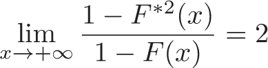
where F *2 = F ′ * F is the cumulative distribution of X1 + X2, the sum of two independent copies of X. This implies that the probability that the sum X1 + X2 exceeds a value x is twice the probability that either one separately exceeds x. Thus, as the threshold grows, an extreme sum is increasingly likely to be driven by a single large value. This is an asymptotic statement, not a claim that every exceedance at a finite threshold has that form.

More generally, it can be shown that the sum of n variables is dominated by the maximum of the values over those variables in the same way. Formally, the following two properties are equivalent to the subexponential condition (see Chistyakov 1964, Embrechts et al. 1979). For a given n ≥ 2, let S n = 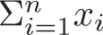and

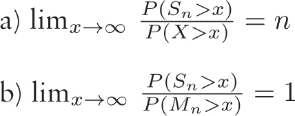
These relations compare the tails of the sum S n and the maximum M n. They describe the importance of a single large value in extreme outcomes, rather than asserting that every observed sum is close to its largest component.

Intuitively, subexponential tails decline more slowly than exponential tails, making a single large value important to the far-tail behavior of the sum. Indeed, one can show that subexponential distributions have no exponential moments:

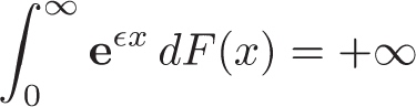
for all values of ε greater than zero. However, the converse isn’t true, since distributions can have no exponential moments, yet not satisfy the subexponential condition.

We note that if we choose to indicate deviations as negative values of the variable x, the same result holds by symmetry for extreme negative values, replacing with . For two-tailed variables, we can separately consider positive and negative domains.

References

- Cramér 1930 — Cramér (1930)
- Teugels 1975 — Teugels (1975)
- Pitman 1980 — Pitman (1980)
- Chistyakov 1964 — Chistyakov (1964)
- Embrechts et al. 1979 — Embrechts et al. (1979)
CONTINUE THE CONVERSATION
Source texts
- Skin In The Game Hidden Asymmetries In Daily Life (Nassim Nicholas Taleb)