Lies, Damned Lies, and Statistics

Lies, Damned Lies, and Statistics

DATA, NUMBERS, AND STATISTICS now have an everyday role in most professional careers, not just in engineering and science. Increasingly, organizations of all kinds are making data-driven decisions. Every field has people studying ways to do it better. Consider K–12 education: What is the most effective way to teach kids to read? How much homework should students be getting? What time of day should school start?

The same is increasingly true in everyday life: What is the best diet? How much exercise is good enough? How safe is this car compared with that one?

Unfortunately, there often aren’t straightforward answers to these types of questions. Instead, there are usually conflicting messages on almost every topic: for nutrition, medicine, government policy (environmental regulation, healthcare, etc.), and the list goes on and on.

For any issue, you can find people on both sides with “numbers” to back up their position. This leads many people to feel that data can be too easily manipulated to support whatever story someone wants to tell, hence the title of this chapter. Similarly, even if people aren’t intentionally trying to mislead you, study results are often accidentally misinterpreted, or the studies themselves can suffer from design flaws.

However, the answer is not to dismiss all statistics or data-driven evidence as nonsense, leaving you to base decisions solely on opinions and guesses. Instead, you must use mental models to get a deeper understanding of an issue, including its underlying research, enabling you to determine what information is credible.

You can also use data from your life and business to derive new insights. Insights based on true patterns, such as those found in market trends, customer behavior, and natural occurrences, can form the basis for major companies and scientific breakthroughs. They can also provide insight in everyday life.

As an example, consider being a first-time parent. Lucky parents have a baby who goes to sleep easily and sleeps through the night at one month old. The rest of us have to hear all the advice: use a rocker, swaddle them, let them cry it out, don’t let them cry it out, co-sleep, change the baby’s diet, change the mother’s diet, and on and on.

Our older son never wanted to be put down, but our pediatrician nevertheless advised us to put him down when he was sleepy but still awake. That always led to him screaming the minute he was set down. If he wasn’t deeply asleep, he would just rouse himself and start crying. The first few nights of this were harrowing, with each of us taking turns staying awake and holding him while he slept; he may have slept on his own for an hour a night.

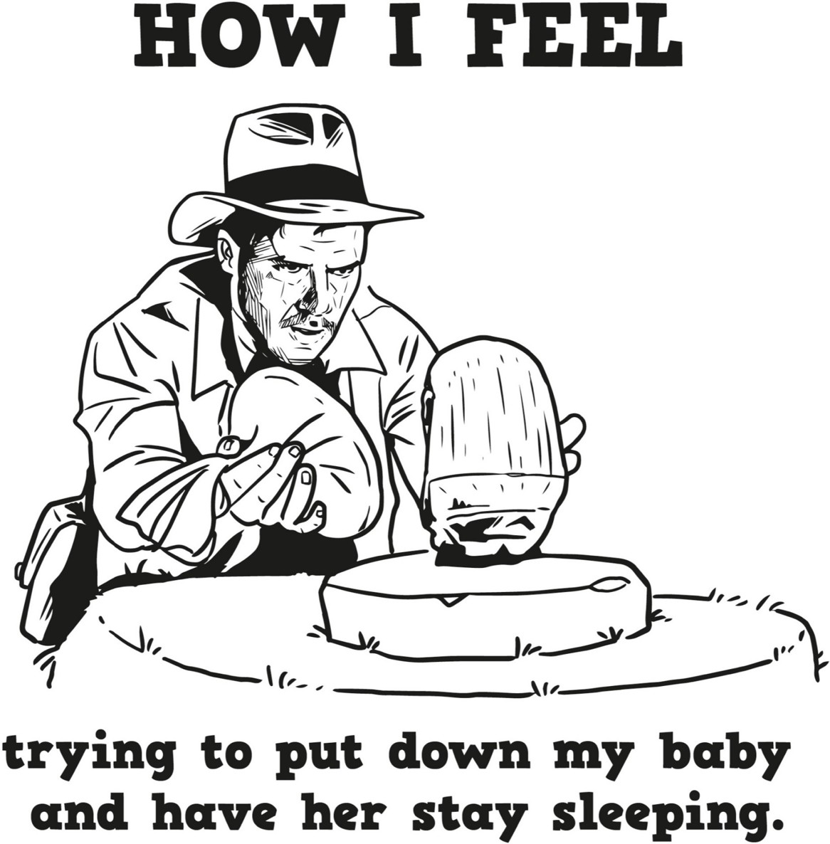
We had to find another way. Through experimentation and collecting our own data over the first few weeks (see scientific method in Chapter 4), we discovered that our son liked a tight swaddle and would fall asleep in an electric swing, preferably on the highest setting. When he grew out of the swaddle, we feared that we were going back to square one. Luckily, he quickly adapted, and before he turned one, he could easily be put down and sleep straight through the night.

When we had our second son, we thought of ourselves as baby-care professionals. We had our magic swing and we thought we were all set. And then, per Murphy’s law (see Chapter 2), baby number two hated the swing. We circled back through all the advice, and after a few days, we tried to set him down when he was sleepy but awake (per our pediatrician’s original advice). Lo and behold, he put himself to sleep!

Like babies and their sleep procedures, many aspects of life have inherent variability and cannot be predicted with certainty. Will it rain today? Which funds should you invest your retirement money in? Who are the best players to draft for your fantasy football team?

Despite this uncertainty, you still have to make a lot of choices, from decisions about your health to deciding whom to vote for to taking a risk with a new project at work. This chapter is about helping you think about wading through such uncertainty in the context of decision making. What advice should you listen to and why?

Probability and statistics are the branches of mathematics that give us the most useful mental models for these tasks. As French mathematician Pierre-Simon Laplace wrote in his 1812 book Théorie Analytique des Probabilités: “The most important questions of life are indeed, for the most part, really only problems of probability.”

We will discuss the useful mental models from the fields of probability and statistics along with common traps to avoid. While many of the basic concepts of probability are fairly intuitive, your intuition often fails you (as we’ve seen throughout this book).

Yes, that means some of this chapter is a bit mathematical. However, we believe that an understanding of these concepts is needed for you to understand the statistical claims that you encounter on a daily basis, and to start to make your own. We’ve tried to include only the level of detail that is really needed to start to appreciate these concepts. And, as always, we’ve included plenty of examples to help you grasp them.

TO BELIEVE OR NOT BELIEVE

It is human nature to use past experience and observation to guide decision making, and evolutionarily this makes sense. If you watched someone get sick after they ate a certain food or get hurt by behaving a certain way around an animal, it follows that you should not copy that behavior. Unfortunately, this shortcut doesn’t always result in good thinking. For example:

We had a big snowstorm this year; so much for global warming.

My grandfather lived to his eighties and smoked a pack a day for his whole life, so I don’t believe that smoking causes cancer.

I have heard several news reports about children being harmed. It is so much more dangerous to be a child these days.

I got a runny nose and cough after I took the flu vaccine, and I think it was caused by the vaccine.

These are all examples of drawing incorrect conclusions using anecdotal evidence, informally collected evidence from personal anecdotes. You run into trouble when you make generalizations based on anecdotal evidence or weigh it more heavily than scientific evidence. Unfortunately, as Michael Shermer, founder of the Skeptics Society, points out in his 2011 book The Believing Brain, “Anecdotal thinking comes naturally, science requires training.”

One issue with anecdotal evidence is that it is often not representative of a full range of experiences. People are more inclined to share out-of-the-ordinary stories. For instance, people are more likely to write a review when they had a terrible experience or an amazing experience. As a result, the only takeaway from an anecdote is that a single event may have occurred.

If you hear an anecdote about someone who smoked and escaped lung cancer, that only proves you are not guaranteed to get lung cancer if you smoke. However, based solely on this anecdote, you cannot draw a conclusion on the chances that an average smoker will get cancer or the relative likelihood of smokers getting lung cancer compared with nonsmokers. If everyone who ever smoked got lung cancer and everyone who didn’t smoke never got lung cancer, the data would be a lot more convincing. Unfortunately, the real world is rarely that simple.

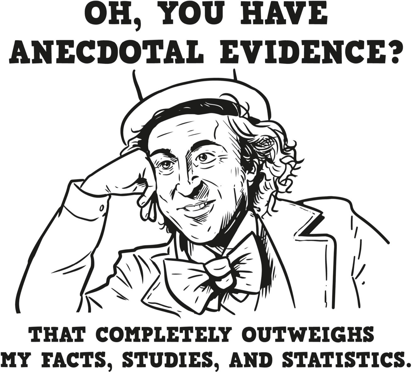
You may have heard anecdotes about people who happened to get cold and flu symptoms around the time that they got the flu vaccine and blame their illness on the vaccine. Just because two events happened in succession, or are correlated, doesn’t mean that the first actually caused the second. Statisticians use the phrase correlation does not imply causation to describe this fallacy.

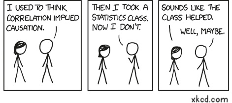
What is often overlooked when this fallacy arises is a confounding factor, a third, possibly non-obvious factor that influences both the assumed cause and the observed effect, confounding the ability to draw a correct conclusion. In the case of the flu vaccine, the cold and flu season is that confounding factor. People get the flu vaccine during the time of year when they are more likely to get sick, whether they have received the vaccine or not. Most likely the symptoms people are experiencing are from a common cold, which the flu vaccine does not protect against.

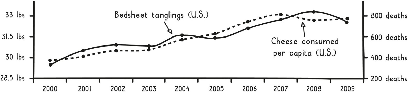
In other instances, a correlation can occur by random chance. It’s easier than ever to test the correlation between all sorts of information, so many spurious correlations are bound to be discovered. In fact, there is a hilarious site (and book) called Spurious Correlations, chock-full of these silly results. The graph below shows one such correlation, between cheese consumption and deaths due to bedsheet tanglings.

Correlation Does Not Imply Causation

One time when Lauren was in high school, she started feeling like a cold was coming on, and her dad told her to drink plenty of fluids to help her get better. She proceeded to drink half a case of raspberry Snapple that day, and, surprisingly, the next day she felt a lot better! Was this clear evidence that raspberry Snapple is a miracle cure for the common cold? No. She probably just experienced a coincidental recovery due to the body’s natural healing ability after also drinking a whole bunch of raspberry Snapple.

Or maybe she wasn’t sick at all; maybe she was just randomly having a bad day, followed by a more regular day. Many purveyors of homeopathic “treatments” include similar anecdotal reports of coincidental recoveries in advertisements for their products. What is not mentioned is what would have happened if there were no “treatment.” After all, even when you are sick, your symptoms will vary day by day. You should require more credible data, such as a thorough scientific experiment, before you believe any medical claims on behalf of a product.

If you set out to collect or evaluate scientific evidence based on an experiment, the first step is to define or understand its hypothesis, the proposed explanation for the effect being studied (e.g., drinking Snapple can reduce the length of the common cold). Defining a hypothesis up front helps to avoid the Texas sharpshooter fallacy. This model is named after a joke about a person who comes upon a barn with targets drawn on the side and bullet holes in the middle of each target. He is amazed at the shooter’s accuracy, only to find that the targets were drawn around the bullet holes after the shots were fired. A similar concept is the moving target, where the goal of an experiment is changed to support a desired outcome after seeing the results.

One method to consider, often referred to as the gold standard in experimental design, is the randomized controlled experiment, where participants are randomly assigned to two groups, and then results from the experimental group (who receive a treatment) are compared with the results from the control group (who do not). This setup isn’t limited to medicine; it can be used in fields such as advertising and product development. (We will walk through a detailed example in a later section.)

A popular version of this experimental design is A/B testing, where user behavior is compared between version A (the experimental group) and version B (the control group) of a site or product, which may differ in page flow, wording, imagery, colors, etc. Such experiments must be carefully designed to isolate the one factor you are studying. The simplest way to do this is to change just one thing between the two groups.

Ideally, experiments are also blinded, so that participants don’t know which group they are in, preventing their conscious and unconscious bias from influencing the results. The classic example is a blind taste test, which ensures that people’s brand affinities don’t influence their choice.

To take the idea of blinding one step further, the people administering the experiment or analyzing the experiment can also remain unaware of which group the participants are in. This additional blinding helps reduce the impact of observer-expectancy bias (also called experimenter bias), where the cognitive biases of the researchers, or observers, may cause them to influence the outcome in the direction they expected.

Unfortunately, experimenter blinding doesn’t completely prevent observer-expectancy bias, because researchers can still bias results in the preparation and analysis of a study, such as by engaging in selective background reading, choosing hypotheses based on preconceived notions, and selectively reporting results.

In medicine, researchers go to great lengths to achieve properly blinded trials. In 2014, the British Medical Journal (BMJ) published a review by Karolina Wartolowska et al. of fifty-three studies that compared an actual surgical intervention with a “sham” surgery, “including the scenario when a scope was inserted and nothing was done but patients were sedated or under general anesthesia and could not distinguish whether or not they underwent the actual surgery.”

These fake surgeries are an example of a placebo, something that the control participants receive that looks and feels like what the experimental participants receive, but in reality is supposed to have no effect. Interestingly, just the act of receiving something that you expect to have a positive effect can actually create one, called the placebo effect.

While placebos have little effect on some things, like healing a broken bone, the placebo effect can bring about observed benefits for numerous ailments. The BMJ review reported that in 74 percent of the trials, patients receiving the fake surgeries saw some improvement in their symptoms, and in 51 percent of the trials, they improved about as much as the recipients of actual surgeries.

For some conditions, there is even evidence to suggest that the placebo effect isn’t purely a figment of the imagination. As an example, placebo “pain relievers” can produce brain activity consistent with the activity produced by actual pain-relieving drugs. For all the parents out there, this is why “kissing a boo-boo” actually can help make it better. Similarly, anticipation of side effects can also result in real negative effects, even with fake treatments, a phenomenon known as the nocebo effect.

One of the hardest things about designing a solid experiment is defining its endpoint, the metric that is used to evaluate the hypothesis. Ideally, the endpoint is an objective metric, something that can be easily measured and consistently interpreted. Some examples of objective metrics include whether someone bought a product, is still alive, or clicked a button on a website.

However, when the concept that researchers are interested in studying isn’t clearly observable or measurable, they must use a proxy endpoint (also called a surrogate endpoint or marker), a measure expected to be closely correlated to the endpoint they would measure if they could. A proxy essentially means a stand-in for something else. Other uses of this mental model include the proxy vote (e.g., absentee ballot) and proxy war (e.g., current conflicts in Yemen and Syria are a proxy war between Iran and Saudi Arabia).

While there is no one objective measure of the quality of a university, every year U.S. News and World Report tries to rank schools against one another using a proxy metric that is a composite of objective measures, such as graduation rates and admission data, along with more subjective measures, such as academic reputation. Other examples of common proxy metrics include the body mass index (BMI), used to measure obesity, and IQ, used to measure intelligence. Proxy metrics are more prone to criticism because they are indirect measures, and all three of these examples have been criticized significantly.

As an example of why this criticism can be valid, consider abnormal heart rhythms (ventricular arrhythmias) that can cause sudden death. Anti-arrhythmic drugs have been developed that prevent ventricular arrhythmias, and so it would seem obvious that these drugs would be expected to prevent sudden death in the patients who take them. But use of these drugs actually leads to a significant increase in sudden death in patients with asymptomatic ventricular arrhythmias after a heart attack. For these patients, the reduced post-treatment rate of ventricular arrhythmias is not indicative of improved survival and is therefore not a good proxy metric.

However, despite the complications that arise when conducting well-run experiments, collecting real scientific evidence beats anecdotal evidence hands down because you can draw believable conclusions. Yes, you have to watch out for spurious correlations and subtle biases (more on that in the next section), but in the end you have results that can really advance your thinking.

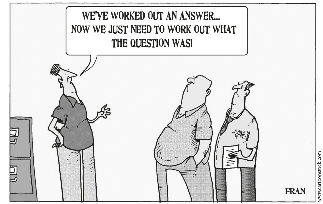
HIDDEN BIAS

In the last section, we mentioned a few things to watch out for when reviewing or conducting experiments, such as observer-expectancy bias and confounding factors. There are a few more of these subtle concepts to be wary of.

First, sometimes it is not ethical or practical to randomly assign people to different experimental groups. For example, if researchers wanted to study the effect of smoking during pregnancy, it wouldn’t be right to make nonsmoking pregnant women start smoking. The smokers in the study would therefore be those who selected to continue smoking, which can introduce a bias called selection bias.

With selection bias, there is no guarantee that the study has isolated smoking to be the only difference between these groups. So if there is a difference detected at the end of the study, it cannot be easily determined how much smoking contributed to this difference. For instance, women who choose to continue smoking during their pregnancy against the advice of doctors may similarly make other medically questionable choices, which could drive adverse outcomes.

Selection bias can also occur when a sample is selected that is not representative of the broader population of interest, as with online reviews. If the group studied isn’t representative, then the results may not be applicable overall.

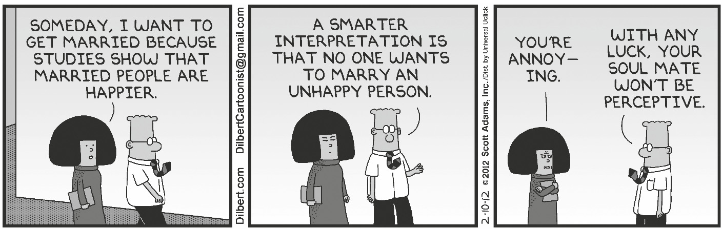
Essentially, you must be really careful when drawing conclusions based on nonrandom experiments. The Dilbert cartoon above pokes fun at the selection bias inherent in a lot of the studies reported in the news.

A similar selection bias occurs with parents and school choice for their kids. Parents understandably want to give their kids a leg up and will often move or pay to send their kids to “better schools.” However, is the school better because there are better teachers or because the students are better prepared due to their parents’ financial means and interest in education? Selection bias likely explains some significant portion of these schools’ better test scores and college admissions.

Another type of selection bias, common to surveys, is nonresponse bias, which occurs when a subset of people don’t participate in an experiment after they are selected for it, e.g., they fail to respond to the survey. If the reason for not responding is related to the topic of the survey, the results will end up biased.

For instance, let’s suppose your company wants to understand whether it has a problem with employee motivation. Like many companies, you might choose to study this potential problem via an employee engagement survey. Employees missing the survey due to a scheduled vacation would be random and not likely to introduce bias, but employees not filling it out due to apathy would be nonrandom and would likely bias the results. That’s because the latter group is made up of disengaged employees, and by not participating, their disengagement is not being captured.

Surveys like this also do not usually account for the opinions of former employees, which can create another bias in the results called survivorship bias. Unhappy employees may have chosen to leave the company, but you cannot capture their opinions when you survey only current employees. Results are therefore biased based on measuring just the population that survived, in this case the employees remaining at the company.

Do these biases invalidate this survey methodology? Not necessarily. Almost every methodology has drawbacks, and bias of one form or another is often unavoidable. You should just be aware of all the potential issues in a study and consider them when drawing conclusions. For example, knowing about the survivorship bias in remaining employees, you could examine the data from exit interviews to see whether motivation issues were mentioned by departing employees. You could even try to survey them too.

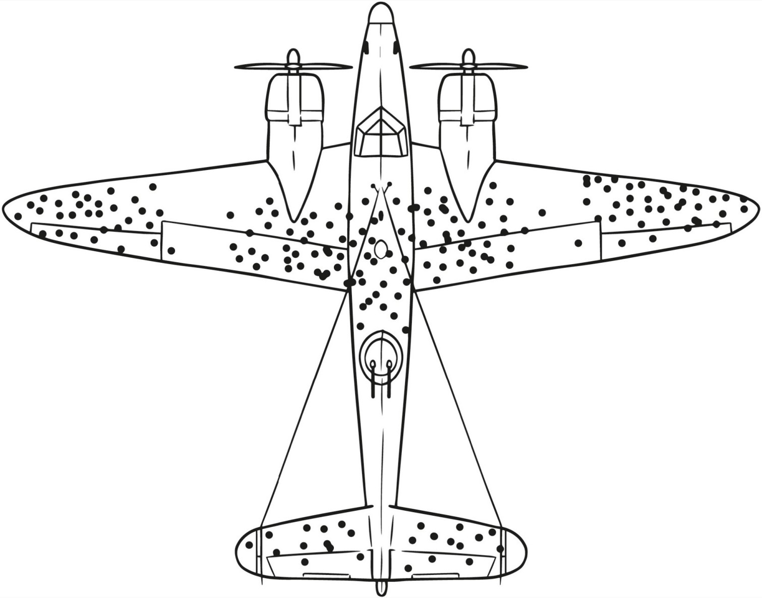
A few other examples can further illustrate how subtle survivorship bias can be. In World War II, naval researchers conducted a study of damaged aircraft that returned from missions, so that they could make suggestions as to how to bolster aircraft defenses for future missions. Looking at where these planes had been hit, they concluded that areas where they had taken the most damage should receive extra armor.

However, statistician Abraham Wald noted that the study sampled only planes that had survived missions, and not the many planes that had been shot down. He therefore theorized the opposite conclusion, which turned out to be correct: that the areas with holes represented areas where aircraft could be shot and still return safely, whereas the areas without holes probably contained areas that, if hit, would cause the planes to go down.

Similarly, if you look at tech CEOs like Bill Gates and Mark Zuckerberg, you might conclude that dropping out of school to pursue your dreams is a fine idea. However, you’d be thinking only of the people that “survived.” You’re missing all the dropouts who did not make it to the top. Architecture presents a more everyday example: Old buildings generally seem to be more beautiful than their modern counterparts. Those buildings, though, are the ones that have survived the ages; there were slews of ugly ones from those time periods that have already been torn down.

Survivorship Bias

When you critically evaluate a study (or conduct one yourself), you need to ask yourself: Who is missing from the sample population? What could be making this sample population nonrandom relative to the underlying population? For example, if you want to grow your company’s customer base, you shouldn’t just sample existing customers; that sample doesn’t account for the probably much larger population of potential customers. This much larger potential customer base may behave very differently from your existing customer base (as is the case with early adopters versus the early majority, which we described in Chapter 4).

One more type of bias that can be inadvertently introduced is response bias. While nonresponse bias is introduced when certain types of people do not respond, for those who do respond, various cognitive biases can cause them to deviate from accurate or truthful responses. For example, in the employee engagement survey, people may lie (by omission or otherwise) for fear of reprisal.

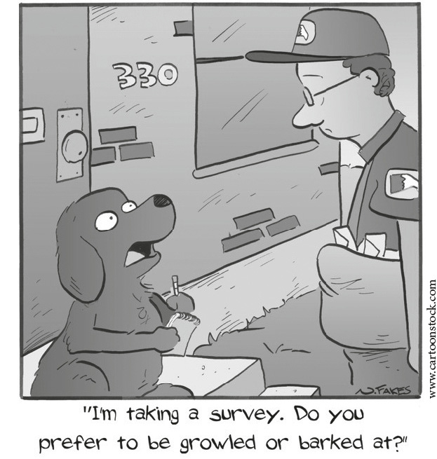
In general, survey results can be influenced by response bias in a number of ways, including the following:

• How questions are worded, e.g., leading or loaded questions
• The order of questions, where earlier questions can influence later ones
• Poor or inaccurate memory of respondents
• Difficulty representing feelings in a number, such as one-to-ten ratings
• Respondents reporting things that reflect well on themselves

It’s worth trying to account for all of these subtle biases (selection bias, nonresponse bias, response bias, survivorship bias), because after you do so, you can be even more sure of your conclusions.

BE WARY OF THE “LAW” OF SMALL NUMBERS

When you interpret data, you should watch out for a basic mistake that causes all sorts of trouble: overstating results from a sample that is too small. Even in a well-run experiment (like a political poll), you cannot expect to get a good estimate based on a small sample. This fallacy is sometimes referred to as the law of small numbers, and this section explores it in more detail. The name is derived from a valid statistical concept called the law of large numbers, which states that the larger the sample, the closer your average result is expected to be to the true average.

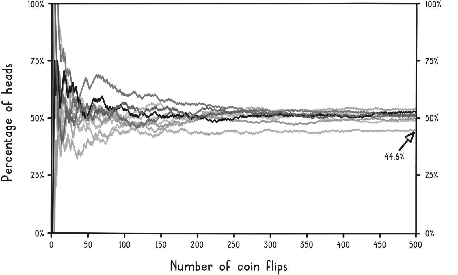
The figure below shows this in action. Each line represents a different series of coin flips and shows how the percentage of heads changes from the first to the five hundredth flip for each series. Note how the curves may deviate quite a bit from the 50 percent mark in the beginning, but start converging closer and closer toward 50 percent as the number of flips increases. But even out to five hundred flips, some of the values are still a fair bit away from 50 percent.

Law of Large Numbers

The speed of convergence for a given experiment depends on the situation. We will explain in a later section how you know when you have a large enough sample. For now, we want to focus on what can go wrong if your sample is too small.

First, consider the gambler’s fallacy, named after roulette players who believe that a streak of reds or blacks from a roulette wheel is more likely to end than to continue with the next spin. Suppose you see ten blacks in a row. Those who fall victim to this fallacy expect the next spin to have a higher chance of coming up red, when in fact the underlying probability of each spin hasn’t changed. For this fallacy to be true, there would have to be some kind of corrective force in the roulette wheel that is bringing the results closer to parity. That’s simply not the case.

It’s sometimes called the Monte Carlo fallacy because in a widely cited case in August 18, 1913, a casino in Monte Carlo had an improbable run of twenty-six blacks! There is only a 1 in 137 million chance of this happening in any twenty-six-ball sequence. However, all other twenty-six-spin sequences are equally rare; they just aren’t all as memorable.

The gambler’s fallacy applies anywhere there is a sequence of decisions, including those by judges, loan officers, and even baseball umpires. In a University of Chicago review of refugee asylum cases from 1985 to 2013, published in the Quarterly Journal of Economics as “Decision-Making Under the Gambler’s Fallacy: Evidence from Asylum Judges, Loan Officers, and Baseball Umpires,” judges were less likely to approve an asylum case if they had approved the last two. It also explains that uncomfortable feeling you might have gotten as a student when you saw that you had chosen answer B four times in a row on a multiple-choice test.

Random data often contains streaks and clusters. Are you surprised to learn that there is a 50 percent chance of getting a run of four heads in a row during any twenty-flip sequence? Streaks like this are often erroneously interpreted as evidence of nonrandom behavior, a failure of intuition called the clustering illusion.

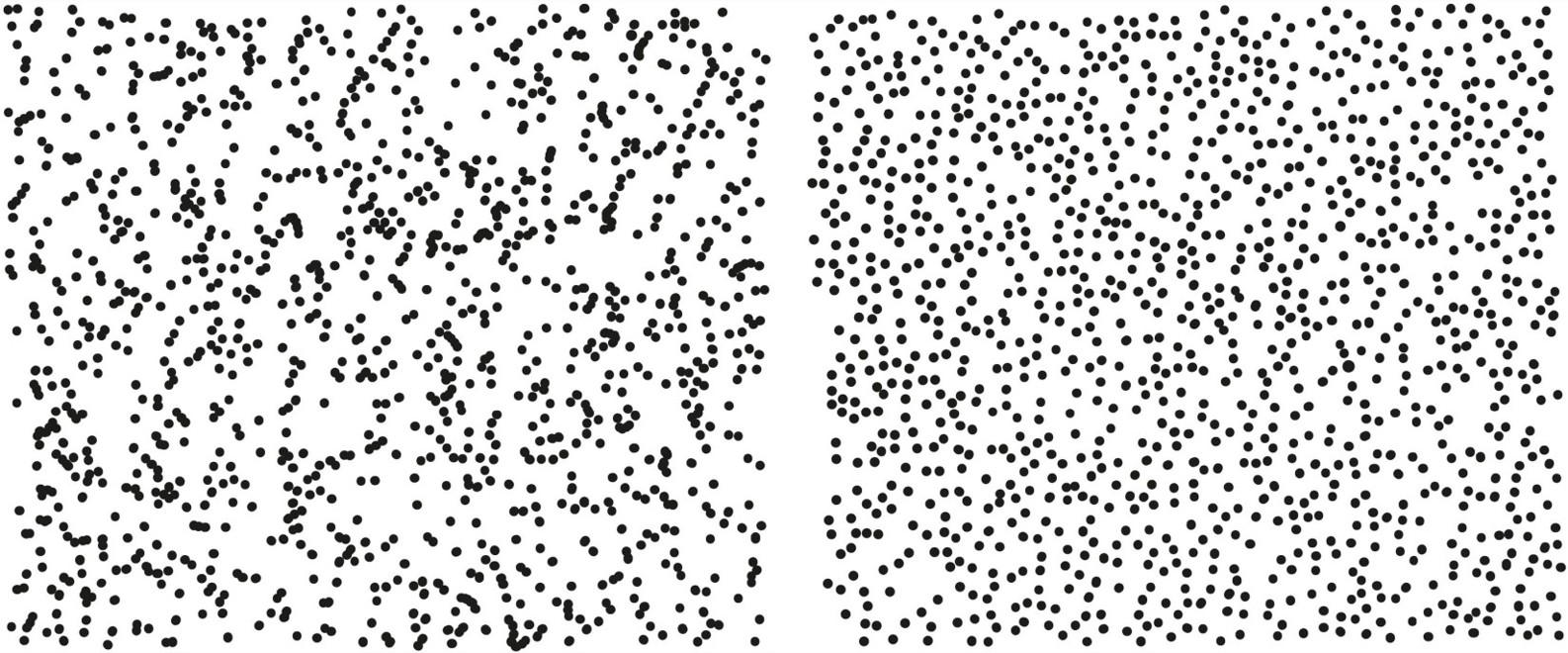
Look at the pair of pictures on the next page. Which is randomly generated?

These pictures come from psychologist Steven Pinker’s book The Better Angels of Our Nature. The left picture—the one with the obvious clusters—is actually the one that is truly random. The right picture—the one that intuitively seems more random—is not; it is a depiction of the positions of glowworms on the ceiling of a cave in Waitomo, New Zealand. The glowworms intentionally space themselves apart from one another in the competition for food.

Clustering Illusion

In World War II, Londoners sought to find a pattern to the bombings of their city by the Germans. Some became convinced that certain areas were being targeted and others were being spared, leading to conspiracy theories about German sympathizers in certain neighborhoods that didn’t get hit. However, statistical analysis showed that there was no evidence to support claims that the bombings were nonrandom.

The improbable should not be confused with the impossible. If enough chances are taken, even rare events are expected to happen. Some people do win the lottery and some people do get struck by lightning. A one-in-a-million event happens quite frequently on a planet with seven billion people.

In the U.S., public health officials are asked to investigate more than one thousand suspected cancer clusters each year. While historically there have been notable cancer clusters caused by exposure to industrial toxins, the vast majority of the cases reported are due to random chance. There are more than 400,000 businesses with fifty or more employees; that’s a lot of opportunities for a handful of people to receive the same unfortunate diagnosis.

Knowing the gambler’s fallacy, you shouldn’t always expect short-term results to match long-term expectations. The inverse is also true: you shouldn’t base long-term expectations on a small set of short-term results.

You might be familiar with the phrase sophomore slump, which describes scenarios such as when a band gets rave reviews for their first album and the second one isn’t as well received, or when a baseball player has a fantastic rookie season but the next year his batting average is not that impressive. In these situations, you may assume there must be some psychological explanation, such as caving under the pressure of success. But in most cases, the true cause is purely mathematical, explained through a model called regression to the mean.

Mean is just another word for average, and regression to the mean explains why extreme events are usually followed by something more typical, regressing closer to the expected mean. For instance, a runner is not expected to follow a record-breaking race with another record-breaking time; a slightly less impressive performance would be expected. That’s because a repeat of a rare result is equally as rare as its first occurrence, such that it shouldn’t be expected the next time.

The takeaway is that you should never assume that a result based on a small set of observations is typical. It may not be representative of either another small set of observations or a much larger set of observations. Like anecdotal evidence, a small sample tells you very little beyond that what happened was within the range of possible outcomes. While first impressions can be accurate, you should treat them with skepticism. More data will help you distinguish what is likely from what is an anomaly.

THE BELL CURVE

When you are dealing with a lot of data, you can use graphs and summary statistics to combat the feeling of information overload (see Chapter 2). The term statistics is actually just the name for numbers used to summarize a dataset. (It also refers to the mathematical process by which those numbers are generated.) Graphs and summary statistics succinctly communicate facts about the dataset.

You use summary statistics all the time without even realizing it. If someone asked you, “What is the temperature of a healthy person?” you’d likely say it was 98.6 degrees Fahrenheit or 37 degrees Celsius. That’s actually a summary statistic called the mean, which, as we just explained, is another word for average.

You probably don’t even remember when you first learned that fact, and it’s even more likely you have no idea where that number comes from. A nineteenth-century German physician, Dr. Carl Wunderlich, diligently collected and analyzed more than a million armpit temperatures from twenty-five thousand patients to calculate that statistic (yes, that’s a lot of armpits).

Yet 98.6 degrees Fahrenheit isn’t some magical temperature. First of all, more recent data indicates a lower mean, closer to 98.2 degrees. Second, you may have noticed from taking your own temperature or that of a family member that “normal” temperatures vary from this mean. In fact, women are slightly warmer than men on average, and temperatures of up to 99.9°F (37.7°C) are still considered normal. Third, people’s temperatures also naturally change throughout the day, moving up on average by 0.9°F (0.5°C) from morning to night.

Just saying a healthy temperature is 98.6°F doesn’t account for all of this nuance. That’s why a range of summary statistics and graphs are often used on a case-by-case basis to summarize data. The mean (average or expected value) measures central tendency, or where the values tend to be centered. Two other popular summary statistics that measure central tendency are the median (middle value that splits the data into two halves) and the mode (the most frequent result). These statistics help describe what a “typical” number might look like for a given set of data.

For body temperature, though, just reporting the central tendency, such as the mean, can at times be too simplistic. This brings us to the second common set of summary statistics, those that measure dispersion, or how far the data is spread out.

The simplest dispersion statistics report ranges. For body temperature, that could be specifying the range of values considered normal, e.g., minimum to maximum reported values from healthy people, as in the graph below (called a histogram).

Histogram

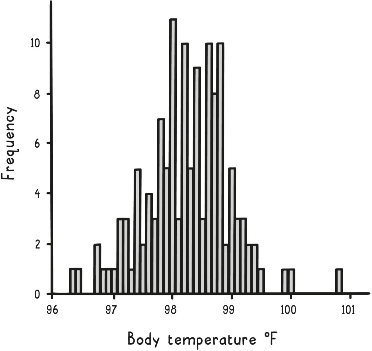
The graph on the previous page depicts the frequencies of 130 different body temperatures derived from a study of healthy adults. A histogram like this one is a simple way that you can summarize data visually: group the values into buckets, count how many data points are in each bucket, and make a vertical bar graph of the buckets.

Before reporting a range, you might first look for outliers, those data points that don’t seem to fit with the rest of the data. These are the data points set apart in the histogram, such as the one at 100.8°F. Perhaps a sick person sneaked into the dataset. As a result, you might report a normal temperature range of 96.3°F to 100.0°F. Of course, with more data, you could produce a more accurate range.

In this dataset, central tendency statistics are quite similar because the distribution of the data is fairly symmetric, with just one peak in the middle. As a result, the mean is 98.25°F, the median is 98.3°F, and the mode is 98°F. In other scenarios, though, these three summary statistics may be quite different.

To illustrate this, consider another histogram, below, showing the distribution of U.S. household income in 2016. This dataset also has one peak, at $20,000–$24,999, but it is asymmetric, skewing to the right. (All incomes above $200,000 are grouped into one bar; had this not been the case, the graph would have a long tail stretching much farther to the right.)

Unlike for the body temperatures, the median income of $59,039 is very different from the mean income of $83,143. Whenever the data is skewed in one direction like this, the mean gets pulled away from the median and toward the skew, swayed by the extreme values.

Distribution of U.S. Household Income (2016)

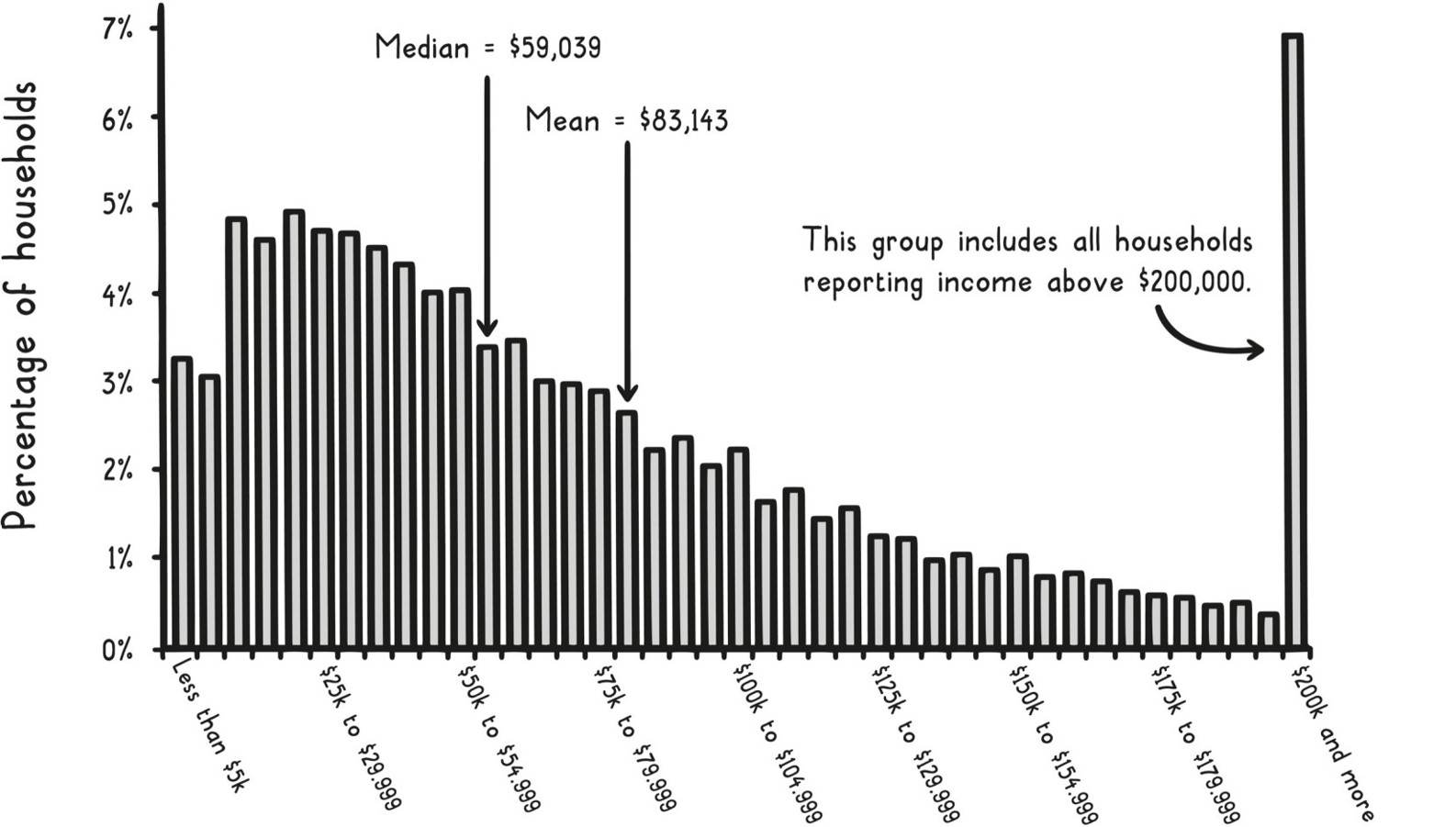
Also, a minimum–maximum range is less informative here. A better summary of the dispersion in this case might be an interquartile range specifying the 25th percentile to the 75th percentile of the data, which captures the middle 50 percent of incomes, from $27,300 to $102,350.

The most common statistical measures of dispersion, though, are the variance and the standard deviation (the latter usually denoted by the Greek letter σ, sigma). They are both measures of how far the numbers in a dataset tend to vary from its mean. The following figure shows how you calculate them for a set of data.

Variance & Standard Deviation

Number of observations: n = 5

Observations: 5, 10, 15, 20, 25

Sample mean: (5+10+15+20+25)/5 = 75/5 = 15

Data point deviations from sample mean, squared:

(5-15)2 = (-10)2 = 100

(10-15)2 = (-5)2 = 25

(15-15)2 = (0)2 = 0

(20-15)2 = (5)2 = 25

(25-15)2 = (10)2 = 100

Sample variance: (100+25+0+25+100)/(n-1) = 250/(5-1) = 250/4 = 62.5

Sample standard deviation (δ): √(variance) = √(62.5) = 7.9

Because the standard deviation is just the square root of the variance, if you know one, then you can easily calculate the other. Higher values for each indicate that it is more common to see data points further from the mean, as shown in the targets below.

Variance

Low Variance

High Variance

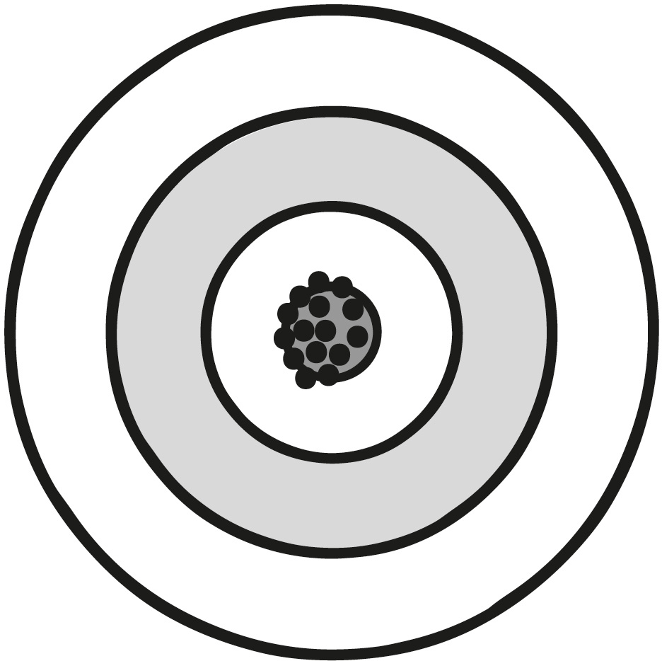
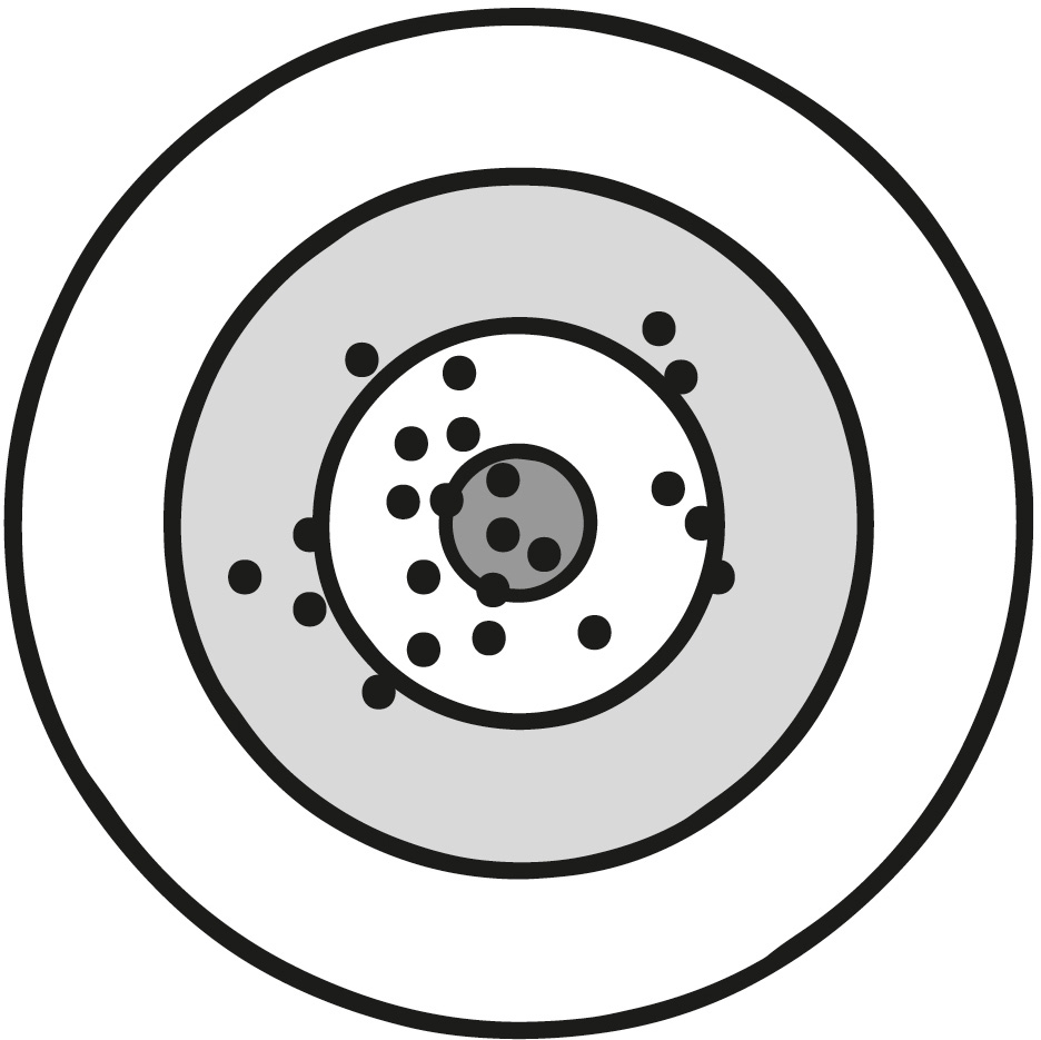
The body temperature dataset depicted earlier has a standard deviation of 0.73°F. Slightly more than two-thirds of its values fall within one standard deviation from its mean (97.52°F to 98.98°F) and 95 percent within two standard deviations (96.79°F to 99.71°F). As you’ll see, this pattern is commonplace for many datasets consisting of measurements (e.g., heights, blood pressure, standardized tests).

Histograms of these types of datasets have similar bell-curve shapes with a cluster of values in the middle, close to the mean, and fewer and fewer results as you go further away from the mean. When a set of data has this type of shape, it is often suggested that it comes from a normal distribution.

The normal distribution is a special type of probability distribution, a mathematical function that describes how the probabilities for all possible outcomes of a random phenomenon are distributed. For example, if you take a random person’s temperature, getting any particular temperature has a certain probability, with the mean of 98.2°F being the most probable and values further away being less and less probable. Given that a probability distribution describes all the possible outcomes, all probabilities in a given distribution add up to 100 percent (or 1).

To understand this better, let’s consider another example. As mentioned above, people’s heights also roughly follow a normal distribution. Below is a graphical representation of the distribution of men’s and women’s heights based on data from the U.S. Centers for Disease Control and Prevention. The distributions both have the typical bell-curve shape, even though the men’s and women’s heights have different means.

Normal Distribution

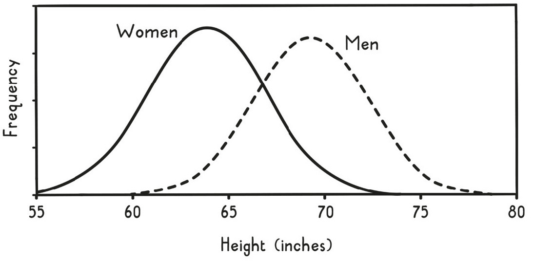
In normal distributions like these (and as we saw with the body temperatures), approximately 68 percent of all values should fall within one standard deviation of the mean, about 95 percent within two, and nearly all (99.7 percent) within three. In this manner, a normal distribution can be uniquely described by just its mean and standard deviation. Because so many phenomena can be described by the normal distribution, knowing these facts is particularly useful.

Normal Distribution Standard Deviations

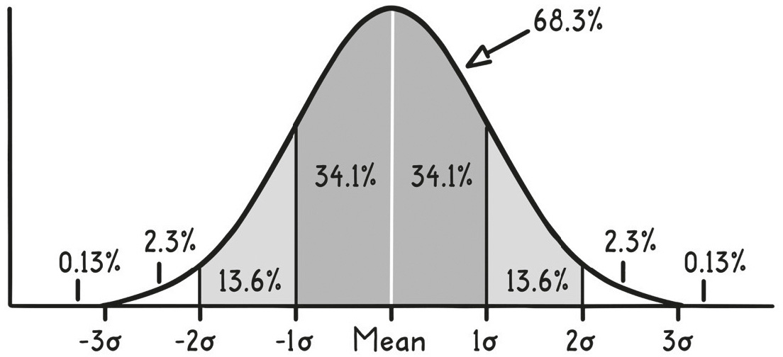
So, if you stopped a random woman on the street, you could use these facts to form a likely guess for her height. A guess of around five feet four inches (162 centimeters) would be best, as that’s the mean. Additionally, you could, with about two-to-one odds, guess that she will have a height between five feet one inch and five feet seven inches. That’s because the standard deviation of women’s heights is slightly less than three inches, so about two-thirds of women’s heights will fall within that range (within one standard deviation of the mean). By contrast, women shorter than four feet ten inches or taller than five feet ten inches make up less than about 5 percent of all women (outside two standard deviations from the mean).

Probability Distributions

Log-normal distribution

Applies to phenomena that follow a power law relationship, such as wealth, the size of cities, and insurance losses.

Poisson distribution

Applies to independent and random events that occur in an interval of time or space, such as lightning strikes or numbers of murders in a city.

Exponential distribution

Applies to the timing of events, such as the survival of people and products, service times, and radioactive particle decay.

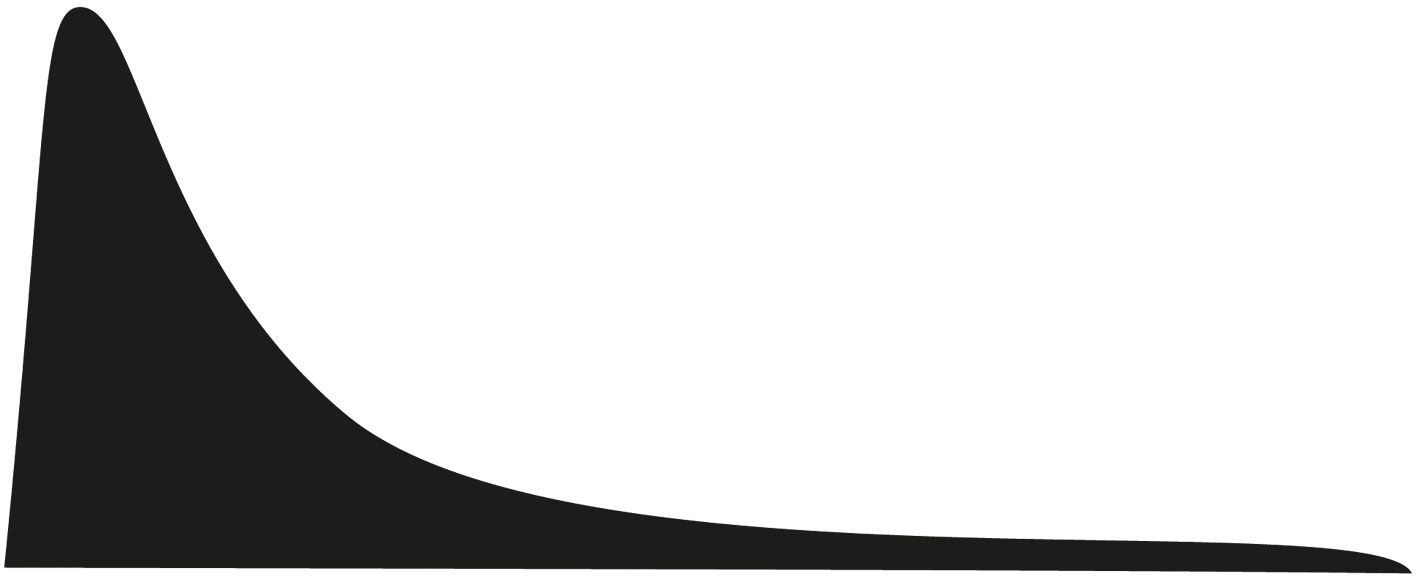
There are many other common probability distributions besides the normal distribution that are useful across a variety of circumstances. A few are depicted in the figure on the previous page.

We called this section “The Bell Curve,” however, because the normal distribution is especially useful due to one of the handiest results in all of statistics, called the central limit theorem. This theorem states that when numbers are drawn from the same distribution and then are averaged, this resulting average approximately follows a normal distribution. This is the case even if the numbers originally came from a completely different distribution.

To appreciate what this theorem means and why it is so useful, consider the familiar opinion poll that determines an approval rating, such as for the U.S. Congress. Each person is asked whether they approve of Congress or not. That means the individual data points are each just a yes or a no.

This type of data looks nothing like a normal distribution, as each data point can take only one of two possible values. Binary data like this is often analyzed using a different probability distribution, called the Bernoulli distribution, which represents the result of a single yes/no-type experiment or question, such as from a survey or poll. This distribution is useful in a wide variety of situations, such as analyzing advertising campaigns (whether someone purchased or not), clinical trials (responded to treatment or not), and A/B testing (clicked or not).

The estimated approval rating is just an average of all of the different individual answers (1 for approval and 0 otherwise). For example, if 1,000 people were polled and 240 approved, then the approval rating would be 24.0 percent. The central limit theorem tells us that this statistical average (sample mean) is approximately normally distributed (assuming enough people participate in the survey). The figure on the next page illustrates how this works visually with the Bernoulli distribution and two others that also initially look nothing like the normal distribution.

The middle column shows how the distribution of the sample mean from a Bernoulli distribution, made up of a series of ones and zeros, ends up looking like a bell curve. The first row depicts a distribution with a 75 percent chance of disapproval (the spike at 0 on the left) and a 25 percent chance of approval (the spike at 1 on the right). This 25 percent chance is based on the approval rating across the whole country, if you polled everyone. Each person in a poll comes from this population distribution.

When you take a poll, you get only an estimate of the overall approval rating (like the 24 percent approval rating estimate mentioned earlier). When you do that, you are taking a sample from the entire population (e.g., asking one thousand people) and averaging the results to calculate the estimate. This sample mean has a distribution itself, called the sample distribution, which describes the chances of getting each possible approval rating from the sample. You can think of this distribution as the result of plotting the different approval ratings (sample means) obtained from many, many polls.

Central Limit Theorem

	Uniform distribution	Bernouli distribution	Exponential distribution
Population distribution	values of x	values of x	values of x
Sample distribution of x average, sample size = 2	values of x average	values of x average	values of x average
Sample distribution of x average, sample size = 5	values of x average	values of x average	values of x average
Sample distribution of x average, sample size = 30	values of x average	values of x average	values of x average

The second row shows a plot of this sample distribution for an approval rating based on polling two randomly selected people. This plot looks different from the original distribution, but still nothing like a normal distribution, as it can have only three outcomes: two approvals (the spike at 1), two disapprovals (the spike at 0), or one approval and one disapproval (the spike at 0.5).

If you base the polls on asking five people, the sample distribution starts to look a bit more like a bell shape with six possible outcomes (third row). With thirty people (thirty-one outcomes, depicted in the fourth row), it starts to look a lot like the characteristic bell-curve shape of the normal distribution.

As you ask more and more people, the sample distribution becomes more and more like a normal distribution, with a mean of 25 percent, the true approval rating from the population distribution. Just as in the case of body temperatures or heights, while this mean is the most likely value obtained by the poll, values close to it are also likely, such as 24 percent. Values further and further away are less and less likely, with probabilities following the normal distribution.

How much less likely, exactly? It depends on how many people you ask. The more people you ask, the tighter the distribution. To convey this information, polls like this usually report a margin of error. An article describing the poll results might include something like “Congress has a 24 percent approval rating with a margin of error of ±3 percent.” The “±3 percent” is the margin of error, but where this margin of error comes from or what it really means is rarely explained. With knowledge of the above mental models, you now can know!

The margin of error is really a type of confidence interval, an estimated range of numbers that you think may include the true value of the parameter you are studying, e.g., the approval rating. This range has a corresponding confidence level, which quantifies the level of confidence you have that the true value of parameter is in the range you estimated. For example, a confidence level of 95 percent tells you that if you ran the poll many times and calculated many confidence intervals (one for each poll), on average 95 percent of them would include the true approval rating (i.e., 25 percent).

Most media reports don’t mention the confidence level used to calculate their margin of error, but it is usually safe to assume they used 95 percent. Research publications, by contrast, are usually more explicit in stating what confidence levels they used to represent the uncertainty in their estimates (again typically, though not always, 95 percent).

For the approval-rating scenario, the range is calculated using the fact that the central limit theorem tells us that the sample mean is approximately normally distributed, so we should expect 95 percent of possible values to be found within two standard deviations of the true mean (i.e., the real approval rating).

The part that hasn’t been explained yet is that the standard deviation of this distribution, also called the standard error, is not the same as the sample standard deviation calculation from earlier. However, these two values are directly related. In particular, the standard error is the same as the standard deviation for the sample, divided by the square root of the sample size. This means that if you want to reduce the margin of error by a factor of two, you need to increase the sample size by a factor of four. For a yes/no poll like the approval rating, a margin of error of 10 percent is achieved with just 96 people, 5 percent at 384 people, 3 percent at 1,067 people, and 2 percent at 2,401. Since the margin of error is an expression of how confident the pollsters are in their estimate, it makes sense that it is directly related to the size of the sample group.

The illustration on the next page shows how confidence intervals work for repeated experiments. It depicts one hundred 95 percent confidence intervals for the probability of flipping heads. Each was calculated from an experiment that involved simulating flipping a fair coin one hundred times. These confidence intervals are represented graphically in the figure by error bars, which are a visual way to display a measure of uncertainty for an estimate.

95% Confidence Intervals from 100 Fair Coin Flips

References

- Théorie Analytique des Probabilités — Pierre-Simon Laplace (1812)
- The Believing Brain — Michael Shermer (2011)
- Sham surgery: a systematic review — Karolina Wartolowska et al. (2014)
- Decision-Making Under the Gambler's Fallacy: Evidence from Asylum Judges, Loan Officers, and Baseball Umpires — University of Chicago review (2013)
- The Better Angels of Our Nature — Steven Pinker (2011)
CONTINUE THE CONVERSATION
Source texts
- Super Thinking (Gabriel Weinberg, Lauren McCann)